1 Probability and Computing 1.9 The Normal Distribution 1.11 The Monte Carlo Method

1.10 Entropy, Randomness, and Information

1.10.1 The Entropy Function

Definition 1.10.1 (Discrete Entropy).

The entropy in bits of a discrete random variable $X$ is

H(X)=-\sum_{x}\Pr\left[X=x\right]\cdot\log_{2}\Pr\left[X=x\right],

where the summation is over the support of $X$ , namely over all values $x$ in the range of $X$ . Equivalently,

H(X)=\operatorname*{\mathbb{E}}\left[\log_{2}\frac{1}{\Pr\left[X\right]}\right].

Definition 1.10.2 (Binary Entropy).

The binary entropy function $H(p)$ for a random variable that assumes only two possible outcomes, one of which occurs with probability $p$ , is

H(p)=-p\log_{2}p-(1-p)\log_{2}(1-p).

Exercise 1.10.3 (Exercise 10.5 [MU17]).

If $p$ is chosen uniformly at random from real interval $[0,1]$ , derive $\operatorname*{\mathbb{E}}\left[H(p)\right]$ .

Proof.

Since $H(p)=-p\log_{2}p-(1-p)\log_{2}(1-p)$ is symmetric, hence we derive the part on the left hand side by

-\int_{0}^{1}p\log_{2}p~{}dp=-\frac{1}{\ln 2}\int_{0}^{1}p\ln p~{}dp=-\frac{1}% {\ln 2}\left(\left.\frac{1}{2}p^{2}\ln p~{}\right|^{1}_{0}-\int^{1}_{0}\frac{1% }{2}p^{2}\cdot\frac{1}{p}~{}dp\right)=\frac{1}{4\ln 2},

where the second equality holds by integration by parts. Therefore, $\operatorname*{\mathbb{E}}\left[H(p)\right]=1/\left(2\ln 2\right)$ . ∎

Exercise 1.10.4 (Exercise 10.2 [MU17]).

Consider an $n$ -sided die, where the $i^{\mathrm{th}}$ face comes up with probability $p_{i}$ . Show that the entropy of a die roll is maximized when each face comes up with equal probability.

Proof.

Let $X$ be the random variable for the face showing up for the $n$ -sided die. The probability of the face showing up can be decided by a set of probabilities $\{p_{i}\}_{i\in I}$ where $\left|I\right|=n-1$ , such that $k\notin I$ and $I\cup\{k\}=[1,n]$ .

On an index $j\in I$ , take partial derivative over $p_{j}$ for $H(X)$ ,

\frac{\partial}{\partial p_{j}}H(X)=-\frac{\partial}{\partial p_{j}}\left(p_{j% }\log_{2}p_{j}\right)-\frac{\partial}{\partial p_{j}}\left(p_{k}\log_{2}p_{k}% \right)=-\frac{1}{\ln 2}\left((\ln p_{j}+1)-(\ln p_{k}+1)\right)=\log_{2}\frac% {p_{k}}{p_{j}},

where $p_{k}=1-\sum_{i\in I}p_{i}$ . By symmetry, $k$ can be arbitrary over $[1,n]$ , hence if the partial derivative is 0 for any pair of $j\neq k$ , the only solution would be $p_{i}=1/n$ for any $i\in[1,n]$ . ∎

Remark 1.10.5.

For a fair $n$ -faced die, the entropy is $\log_{2}n$ bits of randomness.

Exercise 1.10.6 (Exercise 10.4 [MU17]).

Let $p_{k}=\left(k\ln^{2}k\right)^{-1}$ , and show that $S=\sum_{k\geq 2}p_{k}$ is finite. Let integer-valued discrete random variable $X$ has distribution $\Pr\left[X=k\right]=p_{k}/S$ for $k\geq 2$ , show that $H(X)$ is unbounded.

Proof.

Let $g(k)=-\left(\ln k\right)^{-1}$ , then $g^{\prime}(k)=\left(k\ln^{2}k\right)^{-1}$ . Hence,

S\leq\int^{\infty}_{\frac{3}{2}}\frac{1}{k\ln^{2}k}~{}dk=\left.\frac{-1}{\ln k% }\right|^{\infty}_{\frac{3}{2}}=\frac{1}{\ln 3-\ln 2},

(1.9)

which is upper bounded by a bounded value. For the entropy, we have

H(X)=\sum_{k\geq 2}\frac{\log_{2}\left(Sk\ln^{2}k\right)}{Sk\ln^{2}k}=\frac{1}% {\ln 2}\sum_{k\geq 2}\frac{\ln\left(Sk\ln^{2}k\right)}{Sk\ln^{2}k}=\frac{1}{% \ln 2}\sum_{k\geq 2}\left(\boxed{\frac{\ln S}{Sk\ln^{2}k}}_{1}+\boxed{\frac{1}% {Sk\ln k}}_{2}+\boxed{\frac{2\ln\ln k}{Sk\ln^{2}k}}_{3}\right).

The sum over the first term is bounded by eq. 1.9 or by definition of $X$ . For the sum over the third term, the sum over the first few terms with $2\leq k<6$ is bounded. For $k\geq 6$ , the sum over the third term is bounded by

\sum_{k\geq 6}\frac{2\ln\ln k}{Sk\ln^{2}k}\leq\frac{2}{S}\int^{\infty}_{5}% \frac{\ln\ln k}{k\ln^{2}k}~{}dk=\frac{2}{S}\int^{\infty}_{\ln 5}\frac{\ln u}{u% ^{2}}~{}du=\frac{2}{S}\left(\left.\frac{-\ln u}{u}\right|^{\infty}_{\ln 5}+% \int^{\infty}_{\ln 5}\frac{1}{u^{2}}~{}du\right)=-\frac{2}{S}\cdot\left.\frac{% \ln u+1}{u}\right|^{\infty}_{\ln 5},

where $u=\ln k$ , and the summation is finitely bounded. The sum over the second term is

\sum_{k\geq 2}\frac{1}{Sk\ln k}\geq\frac{1}{S}\int^{\infty}_{2}\frac{1}{k\ln k% }~{}dk=\frac{1}{S}\int^{\infty}_{\ln 2}\frac{1}{u}~{}du=\left.\frac{1}{S}\ln u% \right|^{\infty}_{\ln 2},

which is unbounded. We conclude that $H(X)$ is unbounded. ∎

Lemma 1.10.7.

Let $X_{1},X_{2}$ be independent random variables, and let $Y=(X_{1},X_{2})$ . Then $H(Y)=H(X_{1})+H(X_{2})$ .

Proof.

Let $X_{1}$ has support $\Omega_{1}$ , and $X_{2}$ has support $\Omega_{2}$ . We show by

	$\displaystyle H(Y)$	$\displaystyle=-\sum_{x_{1}\in\Omega_{1},x_{2}\in\Omega_{2}}\Pr\left[X_{1}=x_{1% },X_{2}=x_{2}\right]\cdot\log_{2}\Pr\left[X_{1}=x_{1},X_{2}=x_{2}\right]$
		$\displaystyle=-\sum_{x_{1}\in\Omega_{1},x_{2}\in\Omega_{2}}\Pr\left[X_{1}=x_{1% }\right]\cdot\Pr\left[X_{2}=x_{2}\right]\cdot\left(\log_{2}\Pr\left[X_{1}=x_{1% }\right]+\log_{2}\Pr\left[X_{2}=x_{2}\right]\right)$
		$\displaystyle=-\sum_{x_{1}\in\Omega_{1},x_{2}\in\Omega_{2}}\left(\Pr\left[X_{1% }=x_{1}\right]\cdot\log_{2}\Pr\left[X_{1}=x_{1}\right]\cdot\Pr\left[X_{2}=x_{2% }\right]+\Pr\left[X_{2}=x_{2}\right]\cdot\log_{2}\Pr\left[X_{2}=x_{2}\right]% \cdot\Pr\left[X_{1}=x_{1}\right]\right)$
		$\displaystyle=-\sum_{x_{1}\in\Omega_{1}}\Pr\left[X_{1}=x_{1}\right]\cdot\log_{% 2}\Pr\left[X_{1}=x_{1}\right]-\sum_{x_{2}\in\Omega_{2}}\Pr\left[X_{2}=x_{2}% \right]\cdot\log_{2}\Pr\left[X_{2}=x_{2}\right]=H(X_{1})+H(X_{2}),$

where the second and the last equality holds by the independence between $X_{1}$ and $X_{2}$ . ∎

Exercise 1.10.8 (Exercise 10.6 [MU17]).

The conditional entropy $H\left(Y\mid X\right)$ is defined by

H\left(Y\mid X\right)=-\sum_{x,y}\Pr\left[X=x,Y=y\right]\cdot\log_{2}\Pr\left[% Y=y\mid X=x\right].

If $Z=(X,Y)$ , show that $H(Z)=H(X)+H(Y\mid X)$ .

Proof.

This can be seen as an extended version of lemma 1.10.7. We show by

	$\displaystyle H(Z)$	$\displaystyle=-\sum_{x,y}\Pr\left[X=x,Y=y\right]\cdot\log_{2}\Pr\left[X=y,Y=y\right]$
		$\displaystyle=-\sum_{x,y}\Pr\left[X=x,Y=y\right]\cdot\left(\log_{2}\Pr\left[X=% x\right]+\log_{2}\Pr\left[Y=y\mid X=x\right]\right)$
		$\displaystyle=-\sum_{x,y}\left(\Pr\left[X=x\right]\cdot\log_{2}\Pr\left[X=x% \right]+\Pr\left[X=x,Y=y\right]\cdot\log_{2}\Pr\left[Y=y\mid X=x\right]\right)$
		$\displaystyle=H(X)+H\left(Y\mid X\right),$

where the third equality holds by summing $\Pr\left[X=x,Y=y\right]$ over $y$ preserves the marginal probability of $X$ . ∎

Corollary 1.10.9 (Chain Rule of Conditional Entropy).

H\left(X_{1},\ldots,X_{n}\right)=\sum_{i\in[1,n]}H\left(X_{i}\mid X_{1},\ldots% ,X_{i-1}\right).

Corollary 1.10.10 (Bayes’ Rule of Conditional Entropy).

H\left(Y\mid X\right)=H\left(X\mid Y\right)+H\left(Y\right)-H\left(X\right).

Definition 1.10.11 (Mutual Information).

The mutual information of a pair of random variables $(X,Y)$ is defined by

I\left(X;Y\right)=H\left(X\right)-H\left(X\mid Y\right)=H\left(Y\right)-H\left% (Y\mid X\right).

Remark 1.10.12.

For mutual information in definition 1.10.11, we can expand the expression by

	$\displaystyle H\left(Y\right)-H\left(Y\mid X\right)$	$\displaystyle=-\sum_{y}\Pr\left[Y=y\right]\cdot\log_{2}\Pr\left[Y=y\right]+% \sum_{x,y}\Pr\left[Y=y,X=x\right]\cdot\log_{2}\Pr\left[Y=y\mid X=x\right]$
		$\displaystyle=-\sum_{x,y}\Pr\left[Y=y,X=x\right]\cdot\log_{2}\Pr\left[Y=y% \right]+\sum_{x,y}\Pr\left[Y=y,X=x\right]\cdot\log_{2}\Pr\left[Y=y\mid X=x\right]$
		$\displaystyle=-\sum_{x,y}\Pr\left[Y=y,X=x\right]\cdot\left(\log_{2}\Pr\left[Y=% y\right]-\log_{2}\Pr\left[Y=y\mid X=x\right]\right)$
		$\displaystyle=-\sum_{x,y}\Pr\left[Y=y,X=x\right]\cdot\left(\log_{2}\Pr\left[Y=% y\right]+\log_{2}\Pr\left[X=x\right]-\log_{2}\Pr\left[Y=y,X=x\right]\right)$
		$\displaystyle=\sum_{x,y}\Pr\left[Y=y,X=x\right]\cdot\log_{2}\frac{\Pr\left[Y=y% ,X=x\right]}{\Pr\left[Y=y\right]\cdot\Pr\left[X=x\right]}.$

Definition 1.10.13 (KL Divergence [KL51]).

The Kullback-Leibler (KL) divergence is a statistical distance defined as

D_{\mathsf{KL}}\left(P\parallel Q\right)=\sum_{x}P(x)\cdot\log_{2}\frac{P(x)}{% Q(x)}.

Remark 1.10.14 (Mutual Information as KL Divergence).

In KL divergence by definition 1.10.13 and mutual information with remark 1.10.12, if we consider $\mathcal{D}_{(X,Y)}$ , that is the joint distribution of $(X,Y)$ , and $\mathcal{D}_{X}\times\mathcal{D}_{Y}$ , which is the marginal distribution of $(X,Y)$ , mutual information fits into KL divergence by

D_{\mathsf{KL}}\left(\mathcal{D}_{(X,Y)}\parallel\mathcal{D}_{X}\times\mathcal% {D}_{Y}\right)=I\left(X;Y\right).

Moreover, we can again expand the expression in remark 1.10.12 by

	$\displaystyle H\left(Y\right)-H\left(Y\mid X\right)$	$\displaystyle=\sum_{x,y}\Pr\left[Y=y,X=x\right]\cdot\log_{2}\frac{\Pr\left[Y=y% ,X=x\right]}{\Pr\left[Y=y\right]\cdot\Pr\left[X=x\right]}$
		$\displaystyle=\sum_{x,y}\Pr\left[Y=y\mid X=x\right]\cdot\Pr\left[X=x\right]% \cdot\log_{2}\frac{\Pr\left[Y=y\mid X=x\right]}{\Pr\left[Y=y\right]}$
		$\displaystyle=\sum_{x}\Pr\left[X=x\right]\cdot\left(\sum_{y}\Pr\left[Y=y\mid X% =x\right]\cdot\log_{2}\frac{\Pr\left[Y=y\mid X=x\right]}{\Pr\left[Y=y\right]}\right)$
		$\displaystyle=\operatorname*{\mathbb{E}}\left[D_{\mathsf{KL}}\left(\mathcal{D}% _{Y\mid X}\parallel\mathcal{D}_{Y}\right)\right],$

where $\mathcal{D}_{Y\mid X}$ is conditional distribution of $Y$ given $X$ with distribution $\mathcal{D}_{X}$ .

Lemma 1.10.15 (Gibbs’ Inequality).

Given 2 distributions $P$ and $Q$ over the same support,

D_{\mathsf{KL}}\left(P\parallel Q\right)\geq 0.

Proof.

By Jensen’s inequality theorem 1.2.5,

\sum_{x\in\Omega}P(x)\cdot\log_{2}\frac{Q(x)}{P(x)}\leq\log_{2}\left(\sum_{x% \in\Omega}P(x)\cdot\frac{Q(x)}{P(x)}\right)=0.

∎

Corollary 1.10.16 (Monotonicity of Conditional Entropy).

H\left(Y\mid X\right)\leq H\left(Y\right).

1.10.2 Entropy and Binomial Coefficients

For lemma 1.7.1, we give a tighter version as follows, to be used soon.

Lemma 1.10.17 (Tighter Stirling’s Formula).

\sqrt{2\pi n}\left(\frac{n}{e}\right)^{n}\leq n!\leq\sqrt{2\pi n}\left(\frac{n% }{e}\right)^{n}\cdot\exp\left(\frac{1}{12n}\right).

Lemma 1.10.18.

For an integer $nq\in[0,n]$ , we have

\frac{2^{nH(q)}}{2\sqrt{n}}\leq\binom{n}{nq}\leq 2^{nH(q)}.

Proof.

We begin with the upper bound. Since

1=\left(q+(1-q)\right)^{n}\geq\binom{n}{nq}q^{nq}(1-q)^{n(1-q)},

then

\log_{2}\binom{n}{nq}\leq-nq\log_{2}q-n(1-q)\log_{2}(1-q)=nH(q).

The lower bound is trivial when $n=1$ , and it is also trivial when $q=0$ or $1$ for $n\geq 2$ . We derive the lower bound for $n\geq 2$ and $q\in(0,1)$ using the following upper and lower bounds by lemma 1.10.17:

	$\displaystyle n!$	$\displaystyle\geq\sqrt{2\pi n}\left(\frac{n}{e}\right)^{n}$
	$\displaystyle(nq)!$	$\displaystyle\leq\sqrt{2\pi nq}\cdot\left(\frac{nq}{e}\right)^{nq}\cdot\exp% \left(\frac{1}{12nq}\right)$
	$\displaystyle\left(n(1-q)\right)!$	$\displaystyle\leq\sqrt{2\pi n(1-q)}\cdot\left(\frac{n(1-q)}{e}\right)^{n(1-q)}% \cdot\exp\left(\frac{1}{12n(1-q)}\right),$

and therefore

\begin{split}\binom{n}{nq}&\geq\frac{1}{\sqrt{2\pi nq(1-q)}}\cdot\exp\left(-% \frac{1}{12nq(1-q)}\right)\cdot\left(\frac{1}{q}\right)^{nq}\cdot\left(\frac{1% }{1-q}\right)^{n(1-q)}\\ &=\frac{2^{nH(q)}}{\sqrt{2\pi nq(1-q)}}\cdot\exp\left(-\frac{1}{12nq(1-q)}% \right).\end{split}

(1.10)

Let $k=q(1-q)$ such that $0<k\leq 1/4$ , then

\frac{d}{dk}\left(\frac{1}{\sqrt{k}}\cdot\exp\left(-\frac{1}{12nk}\right)% \right)=-\frac{1}{2k^{3/2}}\cdot\exp\left(-\frac{1}{12nk}\right)+\frac{1}{% \sqrt{k}}\cdot\exp\left(-\frac{1}{12nk}\right)\cdot\frac{1}{12nk^{2}}=\frac{1}% {k^{3/2}}\cdot\exp\left(-\frac{1}{12nk}\right)\cdot\left(\frac{1}{12nk}-\frac{% 1}{2}\right),

which is negative for $k\geq\left(6n\right)^{-1}$ , and $k\geq(n-1)/n^{2}\geq\left(6n\right)^{-1}$ when $q\in(0,1)$ , so eq. 1.10 is minimized when $k=1/4$ , giving

\binom{n}{nq}\geq\frac{2^{nH(q)}}{\sqrt{\pi n/2}}\cdot\exp\left(-\frac{1}{3n}% \right).

Moreover,

\left(\frac{2\sqrt{n}}{\sqrt{\pi n/2}}\right)\cdot\exp\left(-\frac{1}{3n}% \right)=\sqrt{\frac{8}{\pi}}\cdot\exp\left(-\frac{1}{3n}\right)>1

for all $n\geq 1$ , then

\binom{n}{nq}\geq\frac{2^{nH(q)}}{2\sqrt{n}}.

∎

Corollary 1.10.19.

When $0\leq q\leq 1/2$ ,

\frac{2^{nH(q)}}{2\sqrt{n}}\leq\binom{n}{\left\lceil nq\right\rceil},\quad% \binom{n}{\left\lfloor nq\right\rfloor}\leq 2^{nH(q)}.

When $1/2\leq q\leq 1$ ,

\frac{2^{nH(q)}}{2\sqrt{n}}\leq\binom{n}{\left\lfloor nq\right\rfloor},\quad% \binom{n}{\left\lceil nq\right\rceil}\leq 2^{nH(q)}.

1.10.3 Entropy: A Measure of Randomness

Definition 1.10.20 (Variable-Length Fair-Bit Extraction Function).

Let $\left|\mathbf{y}\right|$ be the number of bits in a sequence of bits $\mathbf{y}$ . An extraction function $\mathsf{Ext}$ takes as input the value of a random variable $X$ , and outputs a sequence of bits. For every sequence of bits $\mathbf{y}$ with $\left|\mathbf{y}\right|=k$ ,

\Pr\left[\mathsf{Ext}\left(X\right)=\mathbf{y}\mid\left|\mathsf{Ext}(X)\right|% =k\right]=2^{-k},

whenever $\Pr\left[\left|\mathsf{Ext}(X)\right|=k\right]>0$ .

Remark 1.10.21.

We can view the input $X$ as the outcomes of $n$ biased coin flips, and the output $\mathbf{y}$ as $k$ fair coin flips. In this sense, if the biased coin comes up heads with probability $p$ , the entropy of the input is $nH(p)$ , which is the maximum possible expected number of fair bits that any extraction function can output.

There is no guarantee that $\mathsf{Ext}$ is efficient (runs in polynomial time).

Example 1.10.22.

Consider a construction of $\mathsf{Ext}$ for $X$ uniformly distributed over $[0,11]$ . The elements in $[0,7]$ can be represented in 3 bits, while we can associate the 4 probabilities in $[8,11]$ with 2 bits. Associate each input $[0,11]$ to each 2 or 3 bit output, such that they output with the same probability. Hence, the probability of outputting 3 bits is $2/3$ , while the probability of outputting 2 bits is $1/3$ , and

\Pr\left[\mathsf{Ext}\left(X\right)=\mathbf{y}\mid\left|\mathsf{Ext}(X)\right|% =k\right]=2^{-k}

for $k$ being 2 or 3, such that definition 1.10.20 is satisfied.

Theorem 1.10.23.

Suppose the value of a random variable $X$ is uniform over $[0,m-1]$ , such that $H\left(X\right)=\log_{2}m$ , then there is an extraction function for $X$ that outputs on average at least $\left\lfloor\log_{2}m\right\rfloor-1=\left\lfloor H(X)\right\rfloor-1$ independent and unbiased bits.

Proof.

Suppose $m$ is a power of 2, the extraction function trivially outputs the value’s $\left\lfloor\log_{2}m\right\rfloor$ bits representation.

In the general case where $m$ is not a power of 2, we first show in an inductive way. Let $\alpha=\left\lfloor\log_{2}m\right\rfloor$ , $Y$ be the random variable for the length of output bits, and for the elements in $[2^{\alpha},m-1]$ , the theorem 1.10.23 still holds, that

\operatorname*{\mathbb{E}}\left[Y\right]\geq\frac{2^{\alpha}}{m}\alpha+\frac{m% -2^{\alpha}}{m}\left(\left\lfloor\log_{2}\left(m-2^{\alpha}\right)\right% \rfloor-1\right)=\alpha-\frac{m-2^{\alpha}}{m}\left(\alpha-\left\lfloor\log_{2% }\left(m-2^{\alpha}\right)\right\rfloor+1\right).

Let $\beta=\left\lfloor\log_{2}\left(m-2^{\alpha}\right)\right\rfloor$ , then since

\frac{2^{\beta+1}}{2^{\beta+1}+2^{\alpha}}\geq\frac{m-2^{\alpha}}{m}\geq\frac{% 2^{\beta}}{2^{\beta}+2^{\alpha}},

we have

\operatorname*{\mathbb{E}}\left[Y\right]\geq\alpha-\frac{m-2^{\alpha}}{m}\left% (\alpha-\beta+1\right)\geq\alpha-\frac{2^{\beta+1}}{2^{\beta+1}+2^{\alpha}}% \left(\alpha-\beta+1\right)=\alpha-\frac{1}{1+2^{\alpha-\beta-1}}\left(\alpha-% \beta+1\right)\geq\alpha-1,

as $2^{\alpha-\beta-1}\geq\alpha-\beta$ holds for any $\alpha>\beta$ .

We show in an explicit construction. Consider $k$ distinct indices $\{\beta_{i}\}_{i\in[1,k]}\subseteq[0,\alpha]$ in descending order, satisfying

m=\sum_{i\in[1,k]}2^{\beta_{i}},\quad s_{i}=\sum_{j\in[1,i]}2^{\beta_{j}},

such that $[0,m-1]$ is partitioned into $k$ subsets, and the $i^{\mathrm{th}}$ subset is $[s_{i-1},s_{i}-1]$ , of size $2^{\beta_{i}}$ , then

\operatorname*{\mathbb{E}}\left[Y\right]=\sum_{i\in[1,k]}\frac{2^{\beta_{i}}}{% m}\beta_{i},

and since $\beta_{1}=\alpha$ ,

\operatorname*{\mathbb{E}}\left[Y\right]-(\alpha-1)=\frac{2^{\beta_{1}}}{m}+% \sum_{i\in[2,k]}\frac{2^{\beta_{i}}}{m}\left(\beta_{i}-(\alpha-1)\right)=\frac% {1}{m}\left(2^{\beta_{1}}-\sum_{i\in[2,k]}2^{\beta_{i}}\left((\alpha-1)-\beta_% {i}\right)\right).

Considering

2^{\beta_{1}}-\sum_{i\in[2,k]}2^{\beta_{i}}\left((\alpha-1)-\beta_{i}\right)% \geq 2^{\alpha}-\sum_{i\in[0,\alpha-2]}2^{i}\cdot\left(\alpha-1-i\right)=2^{% \alpha}-\left(\left(2^{\alpha}-1\right)-\alpha\right)=\alpha+1>0,

then $\operatorname*{\mathbb{E}}\left[Y\right]>\alpha-1$ . ∎

Exercise 1.10.24 (Exercise 10.9 [MU17]).

We have shown in theorem 1.10.23 that an extraction function for a random variable $X$ uniform over $[0,m-1]$ extracts on average at least $\left\lfloor H(X)\right\rfloor-1$ unbiased bits. Show that there is an extraction function for $\{X_{i}\}_{i\in[1,k]}$ independent random variables uniform over $[0,m-1]$ extracting on average at least $k\left\lfloor H(X)\right\rfloor-1$ unbiased bits.

Proof.

Apparently, one can invoke $k$ times the extraction function in theorem 1.10.23, and by linearity of expectation, outputting on average at least $k\left\lfloor H(X)\right\rfloor-k$ unbiased bits. The idea is to construct $W$ over $[0,m^{k}-1]$ by

W=X_{1}+mX_{2}+m^{2}X_{3}+\cdots+m^{k-1}X_{k},

and $H(W)=H\left(X_{1},\ldots,X_{k}\right)=k\log_{2}m$ . The average number of output bits by theorem 1.10.23 is

\left\lfloor k\log_{2}m\right\rfloor-1\geq k\left\lfloor\log_{2}m\right\rfloor% -1.

∎

Exercise 1.10.25 (Exercise 10.10 [MU17]).

Suppose we have an oracle of generating independent fair coin flips, and $m$ is not a power of 2.

•

Show that one cannot uniformly sample over $[0,m-1]$ with exactly $k$ fair coin flips, for any fixed $k$ .
•

Show that one cannot uniformly sample over $[0,m-1]$ with at most $k$ fair coin flips, for any fixed $k$ .
•

Give an algorithm using fair coins to sample uniformly over $[0,m-1]$ , with expected flips at most $2\left\lceil\log_{2}m\right\rceil$ .

Proof.

We first rule out the case that $2^{k}<m$ , as it is impossible to associate $2^{k}$ outcomes with $m$ numbers.

If one tries to uniformly sample over $[0,m-1]$ with exactly $k$ fair coins, $m\not\mid 2^{k}$ as $m$ is not a power of 2, and one cannot associate $m$ numbers with $2^{k}$ outcomes in an equal-sized partition manner.

In the at most $k$ flips case, pad each execution to exactly $k$ flips: if the algorithm stops after $\ell$ flips with $\ell<k$ , then all $2^{k-\ell}$ possible continuations are counted as producing the same outcome. Hence each output $a$ corresponds to some integer number $N_{a}$ of the $2^{k}$ length- $k$ bit strings, so

\Pr\left[\text{outputting }a\right]=N_{a}\cdot 2^{-k}.

Uniformity requires $N_{a}/2^{k}=1/m$ for every $a$ , so $m\mid 2^{k}$ , which is impossible because $m$ is not a power of $2$ , failing in the same manner as the exact $k$ tosses.

An algorithm sampling uniformly over $[0,m-1]$ is rejection sampling: keep tossing $\left\lceil\log_{2}m\right\rceil$ fair coins, until the outputting integer is within range $[0,m-1]$ . A round being rejected has probability at most $1/2$ , and the expected number of rounds is therefore at most 2, thus the expected runtime is at most $2\left\lceil\log_{2}m\right\rceil$ . ∎

Exercise 1.10.26 (Exercise 10.11 [MU17]).

Suppose we have an oracle of generating independent fair coin flips.

•

Give an algorithm using the fair coin that simulates flipping a biased coin that comes up heads with probability $p$ . The expected number of flips should be at most 2.
•

Give an algorithm using the coin to sample uniformly over $[0,m-1]$ with expected flips at most $\left\lceil\log_{2}m\right\rceil+2$ .

Proof.

Write $p$ into its binary form, such that there exists bits $\{b_{i}\}_{i\geq 1}$ , to binary decompose $p$ into the form $\sum_{i\geq 1}b_{i}/2^{i}$ . Keep tossing independent fair coins $\{X_{i}\}_{i\geq 1}$ until $X_{i}\neq b_{i}$ . If $X_{i}>b_{i}$ , the biased coin comes up tails, otherwise heads. Since $\Pr\left[X_{i}\neq b_{i}\right]=1/2$ , the expected number of sampling is at most 2, as there might be finite number of $\{b_{i}\}_{i\geq 1}$ .

A first attempt at sampling uniformly over $[0,m-1]$ is an extension of the biased coin sampling, with probability $m/2^{\alpha}$ the biased coin comes up heads, where $\alpha=\left\lceil\log_{2}m\right\rceil$ . In each attempt, fair coins are tossed sequentially, and they are used both to simulate the biased coin, and maintained as the prefix of an $\alpha$ -bit integer.

•

If the biased coin comes up tails, then any completion of the current prefix ties to an integer at least $m$ , so restart.
•

If the biased coin comes up heads, the generated number is within $[0,m-1]$ ; keep tossing until $\alpha$ fair coins have been sampled, and output the resulting $\alpha$ -bit integer.

Let $A_{i}=(Y_{i},Z_{i})$ be the random variable for the $i^{\mathrm{th}}$ biased coin simulation, where $Y_{i}$ is the number of fair coins tossed, and $Z_{i}$ is the outcome of the biased coin simulation. Let $T$ be a stopping time for $A_{1},A_{2},\ldots$ on the first heads of the biased coin. Then the total number of fair coin flips is

W=\sum_{i\in[1,T]}Y_{i}+\left(\alpha-Y_{T}\right)=\sum_{i\in[1,T-1]}Y_{i}+\alpha.

Since $Z_{i}$ is heads with probability $m/2^{\alpha}$ , then $\operatorname*{\mathbb{E}}\left[T\right]=2^{\alpha}/m\leq 2$ . Moreover, for each $Y_{i}$ ,

\operatorname*{\mathbb{E}}\left[Y_{i}\right]=\sum_{k\in[1,\alpha]}\frac{k}{2^{% k}}+\frac{\alpha}{2^{\alpha}}=2-\frac{2}{2^{\alpha}}.

Since $\operatorname*{\mathbb{E}}\left[T\right]$ and $\operatorname*{\mathbb{E}}\left[Y_{i}\right]$ are both bounded, by theorem 1.13.18,

\operatorname*{\mathbb{E}}\left[\sum_{i\in[1,T]}Y_{i}\right]=\operatorname*{% \mathbb{E}}\left[Y_{i}\right]\cdot\operatorname*{\mathbb{E}}\left[T\right]=% \frac{2^{\alpha}}{m}\cdot\left(2-\frac{2}{2^{\alpha}}\right).

By linearity of expectation,

\operatorname*{\mathbb{E}}\left[W\right]=\frac{2^{\alpha}}{m}\cdot\left(2-% \frac{2}{2^{\alpha}}\right)+\alpha-\operatorname*{\mathbb{E}}\left[Y_{T}\right% ]\leq\alpha+2\cdot\frac{2^{\alpha}-1}{m}-1\leq\alpha+3

where the second inequality holds by $\operatorname*{\mathbb{E}}\left[Y_{T}\right]\geq 1$ , and the last inequality holds by $2^{\alpha-1}<m\leq 2^{\alpha}$ .

This falls short of the desired $\alpha+2$ bound, because rejected attempts discard all previously sampled bits. We now give a recycling version that keeps the remaining randomness after rejection. Consider the following algorithm:

•
Let $c\leftarrow 0$ and $v\leftarrow 1$ . Keep looping:
- –
  
  Sample $b\stackrel{{\scriptstyle\textsc{r}}}{{\leftarrow}}\{0,1\}$ , and update $c\leftarrow c\times 2+b$ , $v\leftarrow v\times 2$ .
- –
  Continue looping if $v<m$ , otherwise if $v\geq m$ :
  - *
    
    If $c\geq m$ , update $c\leftarrow c-m$ , $v\leftarrow v-m$ .
  - *
    
    Otherwise, output $c$ .

The invariant here is $c$ is always uniform over $[0,v-1]$ , and the algorithm is rejection sampling over $[0,m-1]$ .

Indeed, if $c$ is uniform over $[0,v-1]$ , then after sampling $b\stackrel{{\scriptstyle\textsc{r}}}{{\leftarrow}}\{0,1\}$ , the value $2c+b$ is uniform over $[0,2v-1]$ . On $v\geq m$ , conditioning on $c<m$ gives a uniform output over $[0,m-1]$ ; conditioning on $c\geq m$ makes $c-m$ uniform over $[0,v-m-1]$ , preserving the invariant.

The new algorithm always runs $\alpha$ steps up to the first comparison against $m$ , then let $T$ be the step for the output. We have the following observation: At the $t^{\mathrm{th}}$ step, we have $2^{t}$ possible bit strings, separated into 2 classes:

•

Resolved prefixes: On reading the prefix of a $t$ -bit string, the algorithm stops at some bit and outputs a sample. Any continuation for a resolved prefix is considered stopped.
•

Unresolved prefixes: The algorithm does not output after consuming all of the $t$ bits as inputs.

Lemma 1.10.27.

After the first $\alpha$ bits, the unresolved prefixes at the $t^{\mathrm{th}}$ step form a possibly empty interval $\left[\left\lfloor 2^{t}/m\right\rfloor m,2^{t}-1\right]$ .

Proof.

We prove by induction. Let $q_{t}=\left\lfloor 2^{t}/m\right\rfloor$ . When $t=\alpha$ , the unresolved prefixes are $\left[m,2^{\alpha}-1\right]$ , since $q_{\alpha}=1$ .

Suppose the claim holds for $t=t^{\prime}$ . After tossing one more fair coin, each unresolved prefix has two continuations, so before the next rejection step the unresolved interval doubles to

\left[2q_{t^{\prime}}m,2^{t^{\prime}+1}-1\right].

Once the algorithm sees an entire block of size $m$ in the interval at the bottom of the interval, the block is removed, as that goes to the new resolved prefixes. Hence the unresolved interval that remains is

\left[q_{t^{\prime}+1}m,2^{t^{\prime}+1}-1\right].

This proves the induction step. ∎

With lemma 1.10.27, we upper bound the number of unresolved prefixes at the $t^{\mathrm{th}}$ step $v_{t}$ by $m$ , and thus

	$\displaystyle\operatorname*{\mathbb{E}}\left[T\right]$	$\displaystyle=\sum_{t\geq 0}\Pr\left[T>t\right]=\alpha+\sum_{t\geq\alpha}\Pr% \left[T>t\right]$
		$\displaystyle=\alpha+\Pr\left[T>\alpha\right]+\sum_{t>\alpha}\Pr\left[T>t\right]$
		$\displaystyle\leq\alpha+\frac{2^{\alpha}-m}{2^{\alpha}}+\sum_{t\geq{\alpha+1}}% \frac{m}{2^{t}}=\alpha+1.$

The last equality can be roughly relaxed to an upper bound of $\alpha+2$ , as $m/2^{t}\leq 1/2$ for $t>\alpha$ , and the sum of the last 2 terms is upper bounded by 2. ∎

Theorem 1.10.28.

Suppose a coin comes up heads with probability $p>1/2$ . For any constant $\delta>0$ and sufficiently large $n$ ,

•

There exists an extraction function that on input sequences of $n$ independent flips, outputs an average of at least $(1-\delta)nH(p)$ independent random bits.
•

The average number of bits output by any extraction function on an input of $n$ independent flips is at most $nH(p)$ .

Proof.

We begin by describing an extraction function that extracts on average at least $(1-\delta)nH(p)$ random bits from $n$ flips of the biased coin. After $n$ flips, the number of heads coming up concentrates around $n p$ , which means the outcome is most likely to be one of the $\binom{n}{np}$ sequences with $n p$ heads up.

Conditioned that $k$ heads coming up, the sequence with $k$ heads is uniformly distributed over all $\binom{n}{k}$ sequences, which can be bijectively mapped to $\left[0,\binom{n}{k}-1\right]$ . We apply the randomness extraction function for uniform random variable in theorem 1.10.23 to extract on average $\left\lfloor\log_{2}\binom{n}{k}\right\rfloor-1$ fair bits. Moreover, by lemma 1.10.18, we bound the number of fair bits within the range of $\left[(1-\delta)nH(q),nH(q)\right]$ , where $q=k/n$ .

We now formalize the derivation of the bounds for the number of fair bits extracted from $n$ flips of biased coins with probability $p$ coming up heads. Let $Z$ be a random variable representing the number of heads flipped, and let $B$ be the random variable representing the bits extracted by the extraction function, then by conditional expectation,

\operatorname*{\mathbb{E}}\left[B\right]=\sum_{x\in[0,n]}\Pr\left[Z=x\right]% \cdot\operatorname*{\mathbb{E}}\left[B\mid Z=x\right],

and by theorem 1.10.23,

\operatorname*{\mathbb{E}}\left[B\mid Z=x\right]\geq\left\lfloor\log_{2}\binom% {n}{x}\right\rfloor-1.

Now consider the fact that the number of heads concentrates around $n p$ , to lower bound the average number of fair bits extracted, we consider only $x\in\left[\left\lceil(p-\varepsilon)n\right\rceil,\left\lfloor(p+\varepsilon)n% \right\rfloor\right]$ , where $\varepsilon\leq\min\left(p-1/2,1-p\right)$ . By monotonicity,

\operatorname*{\mathbb{E}}\left[B\mid Z=x\right]\geq\left\lfloor\log_{2}\binom% {n}{x}\right\rfloor-1\geq\left\lfloor\log_{2}\binom{n}{\left\lfloor n(p+% \varepsilon)\right\rfloor}\right\rfloor-1=\operatorname*{\mathbb{E}}\left[B% \mid Z=\left\lfloor n(p+\varepsilon)\right\rfloor\right].

(1.11)

By standard Chernoff’s bound, let $\gamma=\varepsilon/p$ and $\mu=np$ ,

\Pr\left[\left|Z-np\right|\geq\varepsilon n\right]\leq\left(\frac{e^{-\gamma}}% {(1-\gamma)^{1-\gamma}}\right)^{\mu}+\left(\frac{e^{\gamma}}{(1+\gamma)^{1+% \gamma}}\right)^{\mu}\leq\exp\left(-\frac{n\varepsilon^{2}}{3p}\right)+\exp% \left(-\frac{n\varepsilon^{2}}{2p}\right).

Alternatively, by KL Divergence driven Chernoff’s bound in 1.4.4,

\Pr\left[\left|Z-np\right|\geq\varepsilon n\right]\leq 2\exp\left(-2n% \varepsilon^{2}\right).

Moreover, we can further lower bound eq. 1.11 by theorem 1.10.23, that

\begin{split}\operatorname*{\mathbb{E}}\left[B\mid Z=\left\lfloor n(p+% \varepsilon)\right\rfloor\right]&\geq\left\lfloor\log_{2}\binom{n}{\left% \lfloor(p+\varepsilon)n\right\rfloor}\right\rfloor-1\geq\log_{2}\binom{n}{% \left\lfloor(p+\varepsilon)n\right\rfloor}-2\\ &\geq\log_{2}\frac{2^{nH(p+\varepsilon)}}{2\sqrt{n}}-2=nH(p+\varepsilon)-\frac% {1}{2}\log_{2}n-3.\end{split}

(1.12)

Therefore,

	$\displaystyle\operatorname*{\mathbb{E}}\left[B\right]$	$\displaystyle\geq\sum_{x\in\left[\left\lceil(p-\varepsilon)n\right\rceil,\left% \lfloor(p+\varepsilon)n\right\rfloor\right]}\Pr\left[Z=x\right]\cdot% \operatorname*{\mathbb{E}}\left[B\mid Z=x\right]$
		$\displaystyle\geq\Pr\left[\left\|Z-np\right\|\leq\varepsilon n\right]\cdot% \operatorname*{\mathbb{E}}\left[B\mid Z=\left\lfloor(p+\varepsilon)n\right% \rfloor\right]$
		$\displaystyle\geq\left(1-2\exp\left(-2n\varepsilon^{2}\right)\right)\cdot\left% (nH(p+\varepsilon)-\frac{1}{2}\log_{2}n-3\right),$

where the last inequality holds by eq. 1.12. We conclude that, for any $\delta>0$ , we have

\operatorname*{\mathbb{E}}\left[B\right]\geq\left(1-\delta\right)nH(p)

for sufficiently small $\varepsilon$ and sufficiently large $n$ .

We now show no extraction function on average obtains more than $nH(p)$ fair bits. Suppose input bits $\mathbf{x}$ occurs with probability $q$ , and the extraction function outputs $\mathbf{y}$ corresponding to input $\mathbf{x}$ , then by definition 1.10.20,

\Pr\left[\mathsf{Ext}\left(X\right)=\mathbf{y}\mid\left|\mathsf{Ext}(X)\right|% =k\right]=2^{-k},

that conditioned the output number of bits from the extraction function is $k$ , the probability of outputting $\mathbf{y}$ is $2^{-k}$ . Hence, for a fixed $\mathbf{y}$ with $k$ bits, the probability of outputting $\mathbf{y}$ is immediate by the probability of outputting $k$ bits,

\Pr\left[\mathsf{Ext}\left(X\right)=\mathbf{y}\right]=\Pr\left[\mathsf{Ext}% \left(X\right)=\mathbf{y},\left|\mathsf{Ext}(X)\right|=k\right]=2^{-k}\cdot\Pr% \left[\left|\mathsf{Ext}(X)\right|=k\right]\leq 2^{-k}.

Moreover, since

\Pr\left[\mathsf{Ext}\left(X\right)=\mathbf{y}\right]\geq\Pr\left[X=\mathbf{x}% \right]=q,

then $q\leq 2^{-k}$ , giving an upper bound on $k\leq-\log_{2}q$ . Therefore,

\operatorname*{\mathbb{E}}\left[B\right]=\sum_{\mathbf{x}}\Pr\left[X=\mathbf{x% }\right]\cdot\operatorname*{\mathbb{E}}\left[B\mid X=\mathbf{x}\right]\leq-% \sum_{\mathbf{x}}\Pr\left[X=\mathbf{x}\right]\cdot\log_{2}\Pr\left[X=\mathbf{x% }\right]=H(X)=nH(p),

where the second inequality is by upper bounding the output length, and the last equality holds by lemma 1.10.7. ∎

Exercise 1.10.29 (Exercise 10.12 [MU17]).

Consider the extraction function $\mathcal{A}$ whose input is a sequence of $n$ independent flips of a coin that comes up heads with probability $p>1/2$ . Break the sequence $X_{1},\ldots,X_{n}$ into $\left\lfloor n/2\right\rfloor$ pairs, such that $A_{i}=(X_{2i-1},X_{2i})$ , and consider the pairs in order. If $A_{i}$ is heads and tails, it outputs a 0; if $A_{i}$ is tails and heads, it outputs a 1; otherwise, move up to the next pair.

•

Show that the bits extracted by $\mathcal{A}$ are independent and unbiased, and the expected number of bits extracted is

$\left\lfloor n/2\right\rfloor 2p(1-p)\approx np(1-p).$
•

We derive another set of flips $Y_{1},\ldots$ from $X_{1},\ldots,X_{n}$ : Let $j, k$ be 1, and repeat until $j>\left\lfloor n/2\right\rfloor$ : If $A_{j}$ is both heads, $Y_{k}$ is heads and increment $j$ and $k$ ; if $A_{j}$ is both tails, $Y_{k}$ is tails and increment $j$ and $k$ ; otherwise increment $j$ .

The intuition here is to take some randomness $\mathcal{A}$ cannot use effectively and reuse it. Show that the bits produced by running $\mathcal{A}$ over $Y_{1},\ldots$ are independent and unbiased, and further argue that they are independent of those produced by running $\mathcal{A}$ over $X_{1},\ldots,X_{n}$ .
•

We derive another set of flips $Z_{1},\ldots,Z_{\left\lfloor n/2\right\rfloor}$ from $X_{1},\ldots,X_{n}$ : $Z_{i}$ is heads if $A_{i}$ is both heads or tails, otherwise tails. Show that the bits produced by running $\mathcal{A}$ over $Z_{1},\ldots,Z_{\left\lfloor n/2\right\rfloor}$ are independent and unbiased, and further argue that they are independent of those produced by running $\mathcal{A}$ over $X_{1},\ldots,X_{n}$ , and $Y_{1},\ldots$ .
•

After we run $\mathcal{A}$ over $Y_{1},\ldots$ and $Z_{1},\ldots,Z_{\left\lfloor n/2\right\rfloor}$ , we can recursively derive two further sequences from each of the sequences, namely $Y_{1},\ldots$ and $Z_{1},\ldots,Z_{\left\lfloor n/2\right\rfloor}$ , in the same way, run $\mathcal{A}$ on those, and so on.

Let $A(p)$ be the average number of bits extracted for each flip in the sequence $X_{1},\ldots,X_{n}$ , in the limit as the length of the sequence $X_{1},\ldots,X_{n}$ goes to infinity. Let $q=1-p$ , and argue that $A(p)$ satisfies the recurrence

$A(p)=pq+\frac{p^{2}+q^{2}}{2}A\left(\frac{p^{2}}{p^{2}+q^{2}}\right)+\frac{1}{% 2}A\left(p^{2}+q^{2}\right).$
•

Show that $H(p)$ satisfies the same recurrence as $A(p)$ .

Proof.

First, for the bits directly extracted by $\mathcal{A}$ , since the $A_{i}$ are mutually independent, and for $A_{i}=(X_{2i-1},X_{2i})$ , the biased coin tosses are mutually independent, each output bit by $\mathcal{A}$ is independent of the others. The probability of a bit sampled by $\mathcal{A}$ being 1 is the same as the probability of a bit sampled by $\mathcal{A}$ being 0; both are $p(1-p)$ , requiring a head and a tail in $A_{i}$ , so the bits are unbiased. Since a bit is output with probability $2p(1-p)$ by $\mathcal{A}$ , by linearity of expectation, the expected number of bits extracted is $\left\lfloor n/2\right\rfloor 2p(1-p)$ .

To show the bits produced by $\mathcal{A}$ over $Y_{1},\ldots$ are independent and unbiased, we first show $Y_{1},\ldots$ are independent. Since $X_{1},\ldots,X_{n}$ are independent, then $A_{1},\ldots,A_{\left\lfloor n/2\right\rfloor}$ are independent. Since the retained $A_{i}$ are both heads or both tails, then $Y_{1},\ldots$ are independent, so are the output by $\mathcal{A}$ over $Y_{1},\ldots$ . To show the outputs by $\mathcal{A}$ from $Y_{1},\ldots$ are unbiased, since each $Y_{i}$ can be modeled by a biased coin with probability $p^{2}/(p^{2}+q^{2})$ coming up heads, applying the same argument for $\mathcal{A}$ producing unbiased bits over $X_{1},\ldots,X_{n}$ , the outputs by $\mathcal{A}$ over $Y_{1},\ldots$ are unbiased.

To show the bits produced by $\mathcal{A}$ over $Y_{1},\ldots$ are independent of the bits produced by $\mathcal{A}$ over $X_{1},\ldots,X_{n}$ , observe that the former uses only the same-faced $A_{i}$ , while the latter uses only the distinct-faced $A_{i}$ . In the latter case, HT and TH are equally likely, and the corresponding $A_{i}$ are independent across index $i$ . In the former case, the same-faced $A_{i}$ are independent across index $i$ , and the values of these $A_{i}$ are independent of the orders of the distinct-faced $A_{i}$ . Hence, the bits extracted by $\mathcal{A}$ over $Y_{1},\ldots$ are independent of the bits extracted by $\mathcal{A}$ over $X_{1},\ldots,X_{n}$ .

To show the bits produced by $\mathcal{A}$ over $Z_{1},\ldots,Z_{\left\lfloor n/2\right\rfloor}$ are independent and unbiased, we show $Z_{1},\ldots,Z_{\left\lfloor n/2\right\rfloor}$ are independent of each other, as $A_{1},\ldots,A_{\left\lfloor n/2\right\rfloor}$ are independent. Each $Z_{i}$ can be modeled by a biased coin coming up heads with probability $p^{2}+q^{2}$ , then the bits extracted by $\mathcal{A}$ are independent and unbiased.

To show the bits produced by $\mathcal{A}$ over $Z_{1},\ldots,Z_{\left\lfloor n/2\right\rfloor}$ are independent of the bits from $\mathcal{A}$ over $X_{1},\ldots,X_{n}$ , for a bit produced by $\mathcal{A}$ over $Z_{1},\ldots,Z_{\left\lfloor n/2\right\rfloor}$ , supposing it is extracted through $(Z_{i},Z_{i+1})$ , which are determined by $(A_{i},A_{i+1})$ , then it is possible that the bit overlaps with the bits extracted over $A_{i}$ and/or $A_{i+1}$ . Since the $A_{i}$ are independent of each other, then all the other bits extracted over $X_{1},\ldots,X_{n}$ are independent of the bit extracted over $(Z_{i},Z_{i+1})$ . Conditioned that the bit extracted over $(Z_{i},Z_{i+1})$ overlaps with the bit extracted from $A_{i}$ , then $A_{i}$ can be HT or TH, the bit extracted from $A_{i}$ can be 0 or 1, and $Z_{i}$ is tails regardless, and thus the bit extracted over $(Z_{i},Z_{i+1})$ is 1, which is independent of the bit extracted from $A_{i}$ . Symmetrically, if the bit extracted over $(Z_{i},Z_{i+1})$ overlaps with the bit extracted over $A_{i+1}$ , the same argument applies, that the bit extracted over $(Z_{i},Z_{i+1})$ is 0.

To show the bits produced by $\mathcal{A}$ over $Z_{1},\ldots,Z_{\left\lfloor n/2\right\rfloor}$ are independent of the bits from $\mathcal{A}$ over $Y_{1},\ldots$ , the strategy is similar to the last independence argument. Supposing a bit is extracted through $(Z_{i},Z_{i+1})$ , determined by $(A_{i},A_{i+1})$ , then by $A_{i}$ being independent of each other, it suffices to only argue that the bit is independent of the bit extracted from $Y_{1},\ldots$ using a $Y_{j}$ that comes from $A_{i}$ or $A_{i+1}$ . Supposing $A_{j}$ is overlapped, regardless of $A_{j}$ being HH or TT, $Z_{j}$ is heads, and the bit extracted from $(Z_{j},Z_{j+1})$ is 0, independent of the bit extracted using $Y_{j}$ . Symmetrically, if the overlap is with the second coordinate, then that coordinate is heads, and the bit extracted from the $Z$ pair is 1.

For $Y_{1},\ldots$ , the biased coin comes up heads with probability $p^{2}/(p^{2}+q^{2})$ , and the expected number of retained $Y_{i}$ is $(p^{2}+q^{2})n/2$ . For $Z_{1},\ldots,Z_{\left\lfloor n/2\right\rfloor}$ , the biased coin has probability $p^{2}+q^{2}$ of coming up heads. For $\mathcal{A}$ directly extracting from $X_{1},\ldots,X_{n}$ , the expected number of bits extracted is $\left\lfloor n/2\right\rfloor 2pq\approx npq$ . Thus, when $n\to\infty$ , the average number of bits extracted per flip approaches

pq+\frac{p^{2}+q^{2}}{2}A\left(\frac{p^{2}}{p^{2}+q^{2}}\right)+\frac{1}{2}A% \left(p^{2}+q^{2}\right).

To show that $A(p)=H(p)$ , we have

	$\displaystyle\frac{p^{2}+q^{2}}{2}H\left(\frac{p^{2}}{p^{2}+q^{2}}\right)$	$\displaystyle=-p^{2}\log_{2}p-q^{2}\log_{2}q+\frac{p^{2}+q^{2}}{2}\log_{2}% \left(p^{2}+q^{2}\right),$
	$\displaystyle\frac{1}{2}H\left(p^{2}+q^{2}\right)$	$\displaystyle=-\frac{p^{2}+q^{2}}{2}\log_{2}\left(p^{2}+q^{2}\right)-pq\log_{2% }\left(2pq\right),$

and finally

	$\displaystyle A\left(p\right)$	$\displaystyle=pq-p^{2}\log_{2}p-q^{2}\log_{2}q-pq\log_{2}\left(2pq\right)$
		$\displaystyle=-p^{2}\log_{2}p-q^{2}\log_{2}q-pq\log_{2}pq$
		$\displaystyle=-(p^{2}+pq)\log_{2}p-(q^{2}+pq)\log_{2}q$
		$\displaystyle=-p\log_{2}p-q\log_{2}q=H\left(p\right).$

∎

Remark 1.10.30.

1.10.29 is called the Peres extractor [Von51, Eli72, Per92]. The von Neumann method [Von51] extracts the bits pairwise from $X_{1},\ldots,X_{n}$ , but throws away the randomness from the structure of the bit string, and there are two leftover sources of randomness: One is the structure of both heads or both tails, which gives $Y_{1},\ldots$ , and the other is the structure of being equal or not, which gives $Z_{1},\ldots,Z_{\left\lfloor n/2\right\rfloor}$ . The von Neumann method took care of the symmetry case of a head and a tail, and the two leftovers are taken care of in the Peres extractor.

Exercise 1.10.31 (Exercise 10.13 [MU17]).

Suppose we only have a biased 6-sided die with entropy $h>0$ instead of a fair coin. Modify the extraction function in theorem 1.10.28 so that it extracts, on average, almost $h$ random bits per roll from a sequence of die rolls.

Proof.

We consider a variant construction based on theorem 1.10.28, where we roll the die $n$ times. Conditioned on seeing $n_{k}$ occurrences of the $k^{\mathrm{th}}$ face, the sequence is uniformly distributed over all

N=\binom{n}{n_{1};n_{2};n_{3};n_{4};n_{5};n_{6}}

sequences. We apply the theorem 1.10.23 extractor to extract the random variable uniform over $[0,N-1]$ .

Let $Z_{k}$ be the random variable for the number of times the $k^{\mathrm{th}}$ face comes up, $p_{k}$ be the probability that the $k^{\mathrm{th}}$ face comes up, and $B$ be the random variable for the bits extracted. Define

\mathcal{T}_{\varepsilon}=\left\{(n_{1},\ldots,n_{6})~{}:~{}\sum_{k\in[1,6]}n_% {k}=n,\text{ and }\forall k\in[1,6],\left|n_{k}-np_{k}\right|\leq\varepsilon n% \right\}.

By conditional expectation,

	$\displaystyle\operatorname*{\mathbb{E}}\left[B\right]$	$\displaystyle=\sum_{n_{1},\ldots,n_{6}}\operatorname*{\mathbb{E}}\left[B\mid Z% _{1}=n_{1},\ldots,Z_{6}=n_{6}\right]\cdot\Pr\left[Z_{1}=n_{1},\ldots,Z_{6}=n_{% 6}\right]$
		$\displaystyle\geq\min_{(n_{1},\ldots,n_{6})\in\mathcal{T}_{\varepsilon}}% \operatorname*{\mathbb{E}}\left[B\mid Z_{1}=n_{1},\ldots,Z_{6}=n_{6}\right]% \cdot\left(1-\sum_{k\in[1,6]}\Pr\left[\left\|Z_{k}-np_{k}\right\|\geq\varepsilon n% \right]\right)$
		$\displaystyle\geq\min_{(n_{1},\ldots,n_{6})\in\mathcal{T}_{\varepsilon}}\left(% \left\lfloor\log_{2}\binom{n}{n_{1};\ldots;n_{6}}\right\rfloor-1\right)\cdot% \left(1-\sum_{k\in[1,6]}\Pr\left[\left\|Z_{k}-np_{k}\right\|\geq\varepsilon n% \right]\right),$

where the second inequality holds by union bounding, and the third inequality holds by theorem 1.10.23.

We now consider a variant of lemma 1.10.18 for the biased 6-sided die.

Lemma 1.10.32.

For integers $\{nq_{i}\}_{i\in[1,6]}$ in $[0,n]$ and $\sum_{i\in[1,6]}q_{i}=1$ , we have

\frac{1}{2n^{5/2}}\cdot 2^{nH(q_{1},\ldots,q_{6})}\leq\binom{n}{nq_{1};\ldots;% nq_{6}}\leq 2^{nH(q_{1},\ldots,q_{6})},

where $H(q_{1},\ldots,q_{6})=-\sum_{i\in[1,6]}q_{i}\log_{2}q_{i}$ .

Proof.

We begin with the upper bound. Since

1=\left(q_{1}+\ldots+q_{6}\right)^{n}\geq\binom{n}{nq_{1};\ldots;nq_{6}}\prod_% {i\in[1,6]}q_{i}^{nq_{i}},

then we complete the upper bound proof by

\log_{2}\binom{n}{nq_{1};\ldots;nq_{6}}\leq-n\sum_{i\in[1,6]}q_{i}\log_{2}q_{i% }=nH\left(q_{1},\ldots,q_{6}\right).

The lower bound is trivial for $n\in[1,6]$ . Let $I\subseteq[1,6]$ be the subset of indices such that $nq_{i}>0$ . By lemma 1.10.17,

n!\geq\sqrt{2\pi n}\left(\frac{n}{e}\right)^{n},\quad(nq_{i})!\leq\sqrt{2\pi nq% _{i}}\left(\frac{nq_{i}}{e}\right)^{nq_{i}}\exp\left(\frac{1}{12nq_{i}}\right),

and therefore

\binom{n}{nq_{1};\ldots;nq_{6}}\geq\left(\frac{1}{\sqrt{2\pi n}}\right)^{\left% |I\right|-1}\cdot\prod_{i\in I}\left(\frac{1}{\sqrt{q_{i}}}\cdot\exp\left(-% \frac{1}{12nq_{i}}\right)\right)\cdot\prod_{i\in I}q_{i}^{-nq_{i}}=\frac{2^{nH% (q_{1},\ldots,q_{6})}}{\left(2\pi n\right)^{(\left|I\right|-1)/2}}\cdot\prod_{% i\in I}\left(\frac{1}{\sqrt{q_{i}}}\cdot\exp\left(-\frac{1}{12nq_{i}}\right)% \right).

By AM-GM inequality,

\prod_{i\in I}q_{i}\leq\left(\frac{1}{\left|I\right|}\sum_{i\in I}q_{i}\right)% ^{\left|I\right|}\leq\left|I\right|^{-\left|I\right|},

then

\binom{n}{nq_{1};\ldots;nq_{6}}\geq\frac{2^{nH(q_{1},\ldots,q_{6})}}{\left(2% \pi n\right)^{(\left|I\right|-1)/2}}\cdot\prod_{i\in I}\left(\frac{1}{\sqrt{q_% {i}}}\cdot\exp\left(-\frac{1}{12nq_{i}}\right)\right)\geq\frac{2^{nH(q_{1},% \ldots,q_{6})}\cdot\left|I\right|^{\left|I\right|/2}}{\left(2\pi n\right)^{(% \left|I\right|-1)/2}}\cdot\prod_{i\in I}\exp\left(-\frac{1}{12nq_{i}}\right).

On the other hand, since each $nq_{i}\geq 1$ for $i\in I$ , then

	$\displaystyle\binom{n}{nq_{1};\ldots;nq_{6}}$	$\displaystyle\geq\frac{2^{nH(q_{1},\ldots,q_{6})}\cdot\left\|I\right\|^{\left\|I% \right\|/2}}{\left(2\pi n\right)^{(\left\|I\right\|-1)/2}}\cdot\prod_{i\in I}\exp% \left(-\frac{1}{12nq_{i}}\right)$
		$\displaystyle\geq\frac{2^{nH(q_{1},\ldots,q_{6})}\cdot\left\|I\right\|^{\left\|I% \right\|/2}}{\left(2\pi n\right)^{(\left\|I\right\|-1)/2}}\cdot\exp\left(-\frac{% \left\|I\right\|}{12}\right)$
		$\displaystyle=\frac{2^{nH(q_{1},\ldots,q_{6})}}{n^{(\left\|I\right\|-1)/2}}\cdot% \sqrt{2\pi}\cdot\left(\frac{\left\|I\right\|}{2\pi\exp\left(1/6\right)}\right)^{% \left\|I\right\|/2},$

and for $\left|I\right|\in[1,6]$ the coefficient

\sqrt{2\pi}\cdot\left(\frac{\left|I\right|}{2\pi\exp\left(1/6\right)}\right)^{% \left|I\right|/2}\geq\frac{1}{2},

which completes the proof. ∎

By the KL-divergence-driven Chernoff bound in 1.4.4,

\Pr\left[\left|Z_{k}-np_{k}\right|\geq\varepsilon n\right]\leq 2\exp\left(-2n% \varepsilon^{2}\right).

Together with lemma 1.10.32,

	$\displaystyle\operatorname*{\mathbb{E}}\left[B\right]$	$\displaystyle\geq\min_{(n_{1},\ldots,n_{6})\in\mathcal{T}_{\varepsilon}}\left(% \left\lfloor\log_{2}\binom{n}{n_{1};\ldots;n_{6}}\right\rfloor-1\right)\cdot% \left(1-\sum_{k\in[1,6]}\Pr\left[\left\|Z_{k}-np_{k}\right\|\geq\varepsilon n% \right]\right)$
		$\displaystyle\geq\min_{(n_{1},\ldots,n_{6})\in\mathcal{T}_{\varepsilon}}\left(% nH\left(q_{1},\ldots,q_{6}\right)-\frac{5}{2}\log_{2}n-3\right)\cdot\left(1-12% \exp\left(-2n\varepsilon^{2}\right)\right),$

where $q_{k}=n_{k}/n$ . Since $H$ is continuous over $[0,1]^{6}$ , there exists a constant $\gamma_{\varepsilon}\to 0$ as $\varepsilon\to 0$ , such that

	$\displaystyle\operatorname*{\mathbb{E}}\left[B\right]$	$\displaystyle\geq\min_{(n_{1},\ldots,n_{6})\in\mathcal{T}_{\varepsilon}}\left(% nH\left(q_{1},\ldots,q_{6}\right)-\frac{5}{2}\log_{2}n-3\right)\cdot\left(1-12% \exp\left(-2n\varepsilon^{2}\right)\right)$
		$\displaystyle\geq\left(n(h-\gamma_{\varepsilon})-\frac{5}{2}\log_{2}n-3\right)% \cdot\left(1-12\exp\left(-2n\varepsilon^{2}\right)\right),$

proving the lower bound.

To show an extraction function extracts on average at most $n h$ fair bits, the idea is similar to the theorem 1.10.28. Let $X$ be the random variable of the outcome of $n$ die rolls, then for an input-output pair $(\mathbf{x},\mathbf{y})$ with $\left|\mathbf{y}\right|=k$ ,

\Pr\left[X=\mathbf{x}\right]\leq\Pr\left[\mathsf{Ext}\left(X\right)=\mathbf{y}% \right]\leq 2^{-k},

the second inequality was discussed in theorem 1.10.28 from the conditional probability and definition 1.10.20, then

k=\operatorname*{\mathbb{E}}\left[B\mid X=\mathbf{x}\right]\leq-\log_{2}\Pr% \left[X=\mathbf{x}\right].

By conditional expectation,

\operatorname*{\mathbb{E}}\left[B\right]=\sum_{\mathbf{x}}\Pr\left[X=\mathbf{x% }\right]\cdot\operatorname*{\mathbb{E}}\left[B\mid X=\mathbf{x}\right]\leq-% \sum_{\mathbf{x}}\Pr\left[X=\mathbf{x}\right]\cdot\log_{2}\Pr\left[X=\mathbf{x% }\right]=H(X)=nh,

where the last equality is from lemma 1.10.7, and we complete the proof. ∎

1.10.4 Entropy: A Limit of Data Compression

Example 1.10.33.

Consider a biased coin that comes up heads with probability $3/4$ . Let HH map to $0$ , HT map to $10$ , TH map to $110$ , and TT map to $111$ . Then on average, the number of bits we use for each pair of flips is

1\cdot\frac{9}{16}+2\cdot\frac{3}{16}+3\cdot\frac{3}{16}+3\cdot\frac{1}{16}=% \frac{27}{16}<2.

This is an example of compression, as on average a biased coin flip can be represented with less than 1 fair coin flip.

Moreover, it is worth noting that this construction allows for breaking a sequence of biased coin flips into pairs, and concatenating the compression results. The result can be uniquely decoded by simply parsing from left to right. For example, 011110 stands for HHTTHT. The construction preserves the property that the bit representation of any pair of coin flips is not a prefix of the bit representation of any other pair of coin flips.

Representations with this property are called prefix codes.

Exercise 1.10.34 (Exercise 10.15 [MU17]).

We wish to compress a sequence of i.i.d. random variables $X_{1},\ldots$ , where each $X_{j}$ takes on one of $n$ possible values, into a prefix code like example 1.10.33. We map the $i^{\mathrm{th}}$ value among all $n$ values to a codeword, which is a sequence of $\ell_{i}$ bits. Prove that the $\ell_{i}$ must satisfy

\sum_{i\in[1,n]}2^{-\ell_{i}}\leq 1.

Proof.

Consider a binary tree of depth $\ell_{\max}=\max\{\ell_{i}\}_{i\in[1,n]}$ , then the length of a codeword is the distance to the root, and a codeword is a prefix of the path to leaves: 0 stands for the left subtree, and 1 stands for the right subtree. For a codeword of length $\ell_{i}$ , there are $2^{\ell_{\max}-\ell_{i}}$ leaves whose root-to-leaf paths begin with that codeword. These sets of leaves are disjoint, since otherwise one codeword would be a prefix of another codeword, contradicting the prefix code property.

Now that every leaf in the binary tree is owned by at most 1 codeword, the number of owned leaves are

\sum_{i\in[1,n]}2^{\ell_{\max}-\ell_{i}}\leq 2^{\ell_{\max}},

which completes the proof. ∎

Remark 1.10.35.

The 1.10.34 is also called Kraft-McMillan inequality [Kra49, Mcm56].

Definition 1.10.36.

A compression function $\mathsf{Com}$ takes as input a sequence of $n$ coin flips, given as an element of $\{H,T\}^{n}$ , and outputs a sequence of bits, such that each input sequence of $n$ flips yields distinct output sequences.

We consider the case of compressing the outcome of a sequence of biased coin flips, similar to theorem 1.10.28.

Theorem 1.10.37.

Suppose a coin comes up heads with probability $p>1/2$ . For any constant $\delta>0$ and $n$ sufficiently large,

•

There exists a compression function $\mathsf{Com}$ such that the expected number of output bits on an input sequence of $n$ independent coin flips is at most $(1+\delta)nH(p)$ .
•

The expected number of output bits by any compression function on an input sequence of $n$ independent coin flips is at least $(1-\delta)nH(p)$ .

Proof.

We begin with the upper bound, with an explicit construction of a compression function.

Let $\varepsilon>0$ be a sufficiently small constant with $p-\varepsilon>1/2$ . On input a sequence of independent coin flips, output the first bit as a flag bit, 0 when the input has at least $\left\lceil n(p-\varepsilon)\right\rceil$ heads, 1 otherwise. When the first flag bit is 1, the compression function translates a head to a 1, and a tail to a 0, which requires $n+1$ bits to output. When the first flag bit is 0, let the number of coin flip sequences be $m$ , and map a sequence to a value in $[0,m-1]$ .

If there are less than $\left\lceil n(p-\varepsilon)\right\rceil$ heads, we upper bound the probability using Chernoff’s bound by

\Pr\left[X-np<-n\varepsilon\right]\leq\left(\frac{e^{-\gamma}}{(1-\gamma)^{1-% \gamma}}\right)^{\mu}\leq\exp\left(-\frac{\mu\gamma^{2}}{2}\right)=\exp\left(-% \frac{n\varepsilon^{2}}{2p}\right),

where $\gamma=\varepsilon/p$ , and $\mu=np$ .

If there are at least $\left\lceil n(p-\varepsilon)\right\rceil$ heads, we upper bound the number of coin flip sequences by

\sum_{k\in\left[\left\lceil n(p-\varepsilon)\right\rceil,n\right]}\binom{n}{k}% \leq\sum_{k\in\left[\left\lceil n(p-\varepsilon)\right\rceil,n\right]}\binom{n% }{\left\lceil n(p-\varepsilon)\right\rceil}\leq\frac{n}{2}\binom{n}{\left% \lceil n(p-\varepsilon)\right\rceil}\leq\frac{n}{2}\cdot 2^{nH(p-\varepsilon)}% =2^{nH(p-\varepsilon)+\log_{2}n-1}\leq 2^{\left\lfloor nH(p-\varepsilon)+\log_% {2}n\right\rfloor},

where the second and the third inequality holds by $p-\varepsilon>1/2$ , and the fourth inequality holds by corollary 1.10.19. Including the flag bit, it takes at most $nH(p-\varepsilon)+\log_{2}n+1$ bits for the sequences with at least $\left\lceil n(p-\varepsilon)\right\rceil$ heads.

Let $B$ be the number of output bits of the compression function. The upper bound of its expectation is

	$\displaystyle\operatorname*{\mathbb{E}}\left[B\right]$	$\displaystyle\leq\exp\left(-\frac{n\varepsilon^{2}}{2p}\right)\cdot(n+1)+\left% (1-\exp\left(-\frac{n\varepsilon^{2}}{2p}\right)\right)\cdot\left(nH(p-% \varepsilon)+\log_{2}n+1\right)$
		$\displaystyle=1+\exp\left(-\frac{n\varepsilon^{2}}{2p}\right)\cdot n+\left(1-% \exp\left(-\frac{n\varepsilon^{2}}{2p}\right)\right)\cdot\left(nH(p)+n\gamma_{% \varepsilon}+\log_{2}n\right)$
		$\displaystyle=1+nH(p)+\boxed{\exp\left(-\frac{n\varepsilon^{2}}{2p}\right)% \cdot n\left(1-H(p)\right)}+\boxed{\left(1-\exp\left(-\frac{n\varepsilon^{2}}{% 2p}\right)\right)\cdot\left(n\gamma_{\varepsilon}+\log_{2}n\right)},$

where the $\gamma_{\varepsilon}$ is a constant similar to the one in 1.10.31, since $H$ is continuous and monotone over $[1/2,1]$ , $\gamma_{\varepsilon}\to 0$ as $\varepsilon\to 0$ . For $\varepsilon$ sufficiently small, when $n$ is sufficiently large, the first boxed term approaches to 0, and the second boxed term is upper bounded by $\delta nH(p)$ for some constant $\delta$ .

We now show the lower bound. It suffices to consider a compression function minimizing the expected output number of bits. We observe a fact: if an input string $\mathbf{s}_{1}$ is more likely than $\mathbf{s}_{2}$ , then the output number of bits on input $\mathbf{s}_{2}$ should be at least as long as the one of $\mathbf{s}_{1}$ . Otherwise, swapping the two outputs decreases the expectation. Since the probability of deriving a specific sequence with $k$ heads is $p^{k}(1-p)^{n-k}$ , it is more likely for a string to have more heads. Hence, by Chernoff’s bound,

\Pr\left[X>\left\lfloor n(p+\varepsilon)\right\rfloor\right]\leq\Pr\left[X-np>% n\varepsilon-1\right]\leq\left(\frac{e^{\gamma}}{(1+\gamma)^{1+\gamma}}\right)% ^{\mu}\leq\exp\left(-\frac{\mu\gamma^{2}}{3}\right)=\exp\left(-\frac{n\left(% \varepsilon-1/n\right)^{2}}{3p}\right),

where $\mu=np$ , $\gamma=\varepsilon/p-1/np$ , and $\varepsilon$ sufficiently small so that $p+\varepsilon<1$ .

Another fact: for a random variable uniform over $[1,m]$ , on average any compression function outputs at least $\log_{2}m-3$ bits. By mapping to $[0,m-1]$ , and let $\ell$ be the first integer that $2+2+4+\ldots+2^{\ell}\geq m$ , hence $\ell\geq\log_{2}m-1$ . Hence, the average output bit of the compression function is at least $\ell-2$ . Averaged over sequences with $\left\lfloor n(p+\varepsilon)\right\rfloor$ heads, the compression function outputs at least

\log_{2}\binom{n}{\left\lfloor n(p+\varepsilon)\right\rfloor}-3\geq\log_{2}% \frac{2^{nH(p+\varepsilon)}}{2\sqrt{n}}-3=nH(p+\varepsilon)-\frac{1}{2}\log_{2% }n-4

bits. By the ordering of an optimal compression function, sequences with fewer heads have average output length at least this large. The expected number of output bits of the compression function is lower bounded by ignoring the strings with more than $\left\lfloor n(p+\varepsilon)\right\rfloor$ heads, then

\left(1-\exp\left(-\frac{n(\varepsilon-1/n)^{2}}{3p}\right)\right)\cdot\left(% nH(p+\varepsilon)-\frac{1}{2}\log_{2}n-4\right).

By choosing a sufficiently small $\varepsilon$ , and then a sufficiently large $n$ , we can lower bound the expected number of output bits to $(1-\delta)nH(p)$ . ∎

Exercise 1.10.38 (Exercise 10.14 [MU17]).

Suppose we only have a biased 6-sided die with entropy $h>0$ instead of a fair coin. Modify the compression function in theorem 1.10.37 so that it compresses a sequence of die rolls to almost $n h$ bits on average.

Proof.

We begin with the lower bound by reusing lemma 1.10.32 and the ideas in 1.10.31 and theorem 1.10.37. Let $Z_{i}$ be the random variable for the number of times the $i^{\mathrm{th}}$ face comes up, $p_{i}$ be the probability that the $i^{\mathrm{th}}$ face comes up, and $B$ be the random variable for the bits of the compression outcome. Recall the $\mathcal{T}_{\varepsilon}$ defined in 1.10.31, by union bound over Chernoff’s bound in 1.4.4,

\Pr\left[\left(Z_{1},\ldots,Z_{6}\right)\in\mathcal{T}_{\varepsilon}\right]=1-% \Pr\left[\left(Z_{1},\ldots,Z_{6}\right)\notin\mathcal{T}_{\varepsilon}\right]% \geq 1-\sum_{i\in[1,6]}\Pr\left[\left|Z_{i}-np_{i}\right|\geq n\varepsilon% \right]\geq 1-12\exp\left(-2n\varepsilon^{2}\right).

Moreover, by previous discussion in theorem 1.10.37, a compression function minimizing the expected output bits outputs fewer bits on inputs that are more likely than the others, then let $(n_{1},\ldots,n_{6})$ be the face counts that

\prod_{i\in[1,6]}p_{i}^{n_{i}}=\max_{(k_{1},\ldots,k_{6})\in\mathcal{T}_{% \varepsilon}}\prod_{i\in[1,6]}p_{i}^{k_{i}},

and conditioned on $(k_{1},\ldots,k_{6})$ , the inputs are uniform over $\binom{n}{k_{1};\ldots;k_{6}}$ sequences, hence within the $\mathcal{T}_{\varepsilon}$ , the compression function outputs at least

\operatorname*{\mathbb{E}}\left[B\mid Z_{1}=k_{1},\ldots,Z_{6}=k_{6}\right]% \geq\log_{2}\binom{n}{n_{1};\ldots;n_{6}}-3\geq\log_{2}\left(\frac{1}{2n^{5/2}% }\cdot 2^{nH(q_{1},\ldots,q_{6})}\right)-3=nH(q_{1},\ldots,q_{6})-\frac{5}{2}% \log_{2}n-4,

where the second inequality holds by lemma 1.10.32, and $q_{i}=n_{i}/n$ . Since this choice maximizes the probability of each individual sequence with these counts, every other sequence in $\mathcal{T}_{\varepsilon}$ is less likely, so its output length is at least the average output length over this type. Then

	$\displaystyle\operatorname*{\mathbb{E}}\left[B\right]$	$\displaystyle\geq\sum_{(k_{1},\ldots,k_{6})\in\mathcal{T}_{\varepsilon}}% \operatorname*{\mathbb{E}}\left[B\mid Z_{1}=k_{1},\ldots,Z_{6}=k_{6}\right]% \cdot\Pr\left[Z_{1}=k_{1},\ldots,Z_{6}=k_{6}\right]$
		$\displaystyle\geq\left(nH(q_{1},\ldots,q_{6})-\frac{5}{2}\log_{2}n-4\right)% \cdot\left(1-12\exp\left(-2n\varepsilon^{2}\right)\right)$
		$\displaystyle=\left(n(h-\gamma_{\varepsilon})-\frac{5}{2}\log_{2}n-4\right)% \cdot\left(1-12\exp\left(-2n\varepsilon^{2}\right)\right),$

where $\gamma_{\varepsilon}$ is a constant such that $\gamma_{\varepsilon}\to 0$ when $\varepsilon\to 0$ as $H$ is continuous over $[0,1]^{6}$ . Hence, for a sufficiently small $\varepsilon$ , and a sufficiently large $n$ , there exists $\delta$ such that the lower bound $(1-\delta)nh$ is proved.

Now for the upper bound, we follow the main architecture of theorem 1.10.28, by introducing a flag bit separating the case where the dice rolling sequence is not in $\mathcal{T}_{\varepsilon}$ and the case where the dice rolling sequence is in $\mathcal{T}_{\varepsilon}$ . If some count deviates too far, then output in its vanilla form where each face is represented in 3 bits. Otherwise, we count the number of possible sequences in $\mathcal{T}_{\varepsilon}$ to be $m$ , and map a sequence to a value in $[0,m-1]$ , and we have

m=\sum_{(k_{1},\ldots,k_{6})\in\mathcal{T}_{\varepsilon}}\binom{n}{k_{1};% \ldots;k_{6}}\leq\left(2\varepsilon n+1\right)^{5}\binom{n}{n_{1};\ldots;n_{6}% }\leq(2\varepsilon n+1)^{5}\cdot 2^{nH(q_{1},\ldots,q_{6})},

where $n_{1},\ldots,n_{6}$ maximizes $\binom{n}{k_{1};\ldots;k_{6}}$ over $\mathcal{T}_{\varepsilon}$ , the last inequality holds by lemma 1.10.32, and $q_{i}=n_{i}/n$ . Hence,

	$\displaystyle\operatorname*{\mathbb{E}}\left[B\right]$	$\displaystyle\leq 1+12\exp\left(-2\varepsilon^{2}n\right)\cdot 3n+\left(\log_{% 2}\left(\left(2\varepsilon n+1\right)^{5}\cdot 2^{nH(q_{1},\ldots,q_{6})}% \right)+1\right)$
		$\displaystyle=2+12\exp\left(-2\varepsilon^{2}n\right)\cdot 3n+5\log_{2}\left(2% \varepsilon n+1\right)+nH(q_{1},\ldots,q_{6})$
		$\displaystyle=2+12\exp\left(-2\varepsilon^{2}n\right)\cdot 3n+5\log_{2}\left(2% \varepsilon n+1\right)+n(h+\gamma_{\varepsilon}),$

Exercise 1.10.39 (Exercise 10.16 [MU17]).

We wish to compress a sequence of i.i.d. random variables $X_{1},\ldots$ , where each $X_{j}$ takes on one of $n$ values. The $i^{\mathrm{th}}$ value occurs with probability $p_{i}$ , where $p_{1}\geq p_{2}\geq\ldots\geq p_{n}$ . The compressed result follows. Let $T_{i}=\sum_{j\in[1,i-1]}p_{j}$ , and let the $i^{\mathrm{th}}$ codeword to be the first $\ell_{i}=\left\lceil\log_{2}(1/p_{i})\right\rceil$ bits of $T_{i}$ . Show that it is a prefix code example 1.10.33. Let $z$ be the average number of bits used for each $X_{j}$ . Show that $H(X)\leq z\leq H(X)+1$ .

Proof.

We observe that, for the binary representation of $p_{i}$ , the first positive bit is the $\ell_{i}^{\mathrm{th}}$ bit. Since the first positive bit is the $i^{\mathrm{th}}$ bit for any value in $\left[2^{-i},2^{-i+1}\right)$ , proving the claim. Moreover, as $p_{1}\geq\ldots\geq p_{n}$ , then $\ell_{1}\leq\ldots\leq\ell_{n}$ , and it suffices to show that any pair of neighboring adjacent codewords does not violate the prefix code property.

On a pair of $T_{i}$ and $T_{i+1}=T_{i}+p_{i}$ , since $T_{i}\leq T_{i}+2^{-\ell_{i}}\leq T_{i}+p_{i}$ , the first $\ell_{i}$ bits are distinct for the $i^{\mathrm{th}}$ and $(i+1)^{\mathrm{th}}$ codeword, proving the prefix code property.

Now for the average number of bits output by the compression function,

z=\sum_{i\in[1,n]}p_{i}\left\lceil\log_{2}(1/p_{i})\right\rceil\geq-\sum_{i\in% [1,n]}p_{i}\log_{2}p_{i}=H(X),

as $\left\lceil\log_{2}(1/p_{i})\right\rceil\geq-\log_{2}p_{i}$ . Moreover, by $\left\lceil\log_{2}(1/p_{i})\right\rceil\leq-\log_{2}p_{i}+1$ , then

z=\sum_{i\in[1,n]}p_{i}\left\lceil\log_{2}(1/p_{i})\right\rceil\leq\sum_{i\in[% 1,n]}p_{i}\left(-\log_{2}p_{i}+1\right)=H(X)+1,

and we proved $H(X)\leq z\leq H(X)+1$ . ∎

Exercise 1.10.40 (Exercise 10.3 [MU17]).

Flip a fair coin repeatedly $X$ times until the first heads occurs. Find $H(X)$ .

Now a friend flips the fair coin repeatedly until the first heads occurs. One wants to determine how many flips required, and is allowed to ask a series of yes-no questions of the following form: give the friend a set of integers, and the friend answers “yes” iff the number of flips is in the set, and “no” otherwise. Find a strategy such that the expected number of questions asked before determining the number of flips is $H(X)$ . Give an intuitive explanation of why one cannot come up with a strategy that would ask fewer than $H(X)$ questions on average.

Proof.

$X$ follows geometrically distributed random variable with success probability $1/2$ , then $\operatorname*{\mathbb{E}}\left[X\right]=2$ , and

H(X)=-\sum_{i\geq 1}\Pr\left[X=i\right]\cdot\log_{2}\Pr\left[X=i\right]=\sum_{% i\geq 1}\frac{1}{2^{i}}\cdot i=2.

Intuitively, on the $k^{\mathrm{th}}$ question, ask if $X=k$ , then the number of questions is same distributed as $X$ . For a strategy, it is impossible to have a same terminating transcript of the yes-no answers from distinct values of $X$ . Moreover, a terminating transcript cannot be continued, as it converges to a single value, ruling out other values, namely other suffixes. Hence, they form a prefix code. By 1.10.39, at least $H(X)=2$ questions are needed on average. ∎

Exercise 1.10.41 (Exercise 10.17 [MU17]).

Arithmetic coding is a standard compression method. In the case where the string to be compressed is a sequence of biased coin flips, it can be described as follows. For a sequence of i.i.d. Bernoulli trials $X_{1},\ldots,X_{n}$ with success probability $1-p$ . The sequences can be ordered lexicographically, so that for $\mathbf{x},\mathbf{y}\in\{0,1\}^{n}$ , we say $\mathbf{x}<\mathbf{y}$ if $x_{i}=0$ and $y_{i}=1$ in the first coordinate $i$ that $x_{i}\neq y_{i}$ . If $z_{\mathbf{x}}$ is the number of zeroes in the string $\mathbf{x}$ , define $p(\mathbf{x})=p^{z_{\mathbf{x}}}(1-p)^{n-z_{\mathbf{x}}}$ , and $q(\mathbf{x})=\sum_{\mathbf{y}<\mathbf{x}}p(\mathbf{y})$ .

•

Suppose we are given $\mathbf{x}$ sequentially, explain how to compute $q(\mathbf{x})$ in $O(n)$ time.
•

Argue that $\left[q(\mathbf{x}),q(\mathbf{x})+p(\mathbf{x})\right)$ are disjoint subintervals over $\left[0,1\right)$ , show that $\overline{X}=(X_{1},\ldots,X_{n})$ can be represented by any point in $\left[q(\overline{X}),q(\overline{X})+p(\overline{X})\right)$ , and a codeword can be chosen in the interval by the first $\left\lceil\log_{2}(1/p(\overline{X}))\right\rceil+1$ bits, such that the codeword is a prefix code.
•

On a codeword, show how to decompress to determine the corresponding $\overline{X}$ .
•

Using a Chernoff’s bound, argue that $\log_{2}(1/p(\overline{X}))$ is close to $nH(p)$ with high probability.

Proof.

To derive $q(\mathbf{x})$ in $O(n)$ , count $i\in[1,n]$ : when $x_{i}=0$ , move forward; otherwise, add $p\prod_{j\in[1,i-1]}q_{j}$ to $q(\mathbf{x})$ , where $q_{j}$ is the probability corresponding to $x_{j}$ . Eventually, one sub-hypercube at a time, and

q(\mathbf{x})=p\sum_{i\in[1,n]}x_{i}\prod_{j\in[1,i-1]}q_{j}.

Let $\mathbf{x}+1$ be defined as adding by 1 to the number with binary representation $\mathbf{x}$ , then $q(\mathbf{x})$ is monotonically increasing for each $\mathbf{x}\in[0,2^{n}-1]$ , such that $\left[q(\mathbf{x}),q(\mathbf{x})+p(\mathbf{x})\right)$ are disjoint, as $q(\mathbf{x}+1)=q(\mathbf{x})+p(\mathbf{x})$ , and $q(\boldsymbol{1})+p(\boldsymbol{1})=1$ .

By 1.10.39, the first positive bit of $p(\mathbf{x})$ is $\ell_{\mathbf{x}}=\left\lceil\log_{2}(1/p(\mathbf{x}))\right\rceil$ , then there exists a dyadic interval of length $2^{-(\ell_{\mathbf{x}}+1)}$ in $\left[q(\mathbf{x}),q(\mathbf{x})+p(\mathbf{x})\right)$ , as $2^{-\ell_{\mathbf{x}}}\leq p(\mathbf{x})$ . The codeword can be chosen by the lower bound of the dyadic interval, requiring $\ell_{\mathbf{x}}+1$ bits. If a codeword $\mathbf{c}_{0}$ is a prefix of a codeword $\mathbf{c}_{1}$ , then $\mathbf{c}_{1}$ in a dyadic interval of $\mathbf{c}_{0}$ , while the exterior intervals are disjoint, which is a contradiction.

Decoding the codeword $c$ is in the reverse order of deriving $q(\mathbf{x})$ : Count $i\in[1,n]$ , and let the left endpoint $a=0$ . If $c\geq a+p\prod_{j\in[1,i-1]}q_{j}$ , the $i^{\mathrm{th}}$ bit is 1, $q_{i}\leftarrow 1-p$ , and add $p\prod_{j\in[1,i-1]}q_{j}$ to $a$ ; otherwise, the $i^{\mathrm{th}}$ bit is 0 and $q_{i}\leftarrow p$ .

Let $Z$ be the number of tails in $[0,n]$ , then $\operatorname*{\mathbb{E}}\left[Z\right]=np$ , and

Y=\log_{2}(1/p(\overline{X}))=-\log_{2}p\cdot Z-\log_{2}(1-p)\cdot(n-Z)=-n\log% _{2}(1-p)+Z\log_{2}\frac{1-p}{p},

such that $\operatorname*{\mathbb{E}}\left[Y\right]=nH(p)$ . If $p=1/2$ , $Y=nH(p)=n$ deterministically. Otherwise, as $Z=\sum_{i\in[1,n]}Z_{i}$ for independent $Z_{i}$ being 1 on the $i^{\mathrm{th}}$ flip, we can apply Chernoff’s bound, such that

\Pr\left[\left|Y-nH(p)\right|\geq\delta np\left|\log_{2}\frac{1-p}{p}\right|% \right]=\Pr\left[\left|Z-np\right|\geq\delta np\right]\leq\left(\frac{e^{% \delta}}{(1+\delta)^{1+\delta}}\right)^{np}+\left(\frac{e^{-\delta}}{(1-\delta% )^{1-\delta}}\right)^{np}\leq 2\exp\left(-\frac{\delta^{2}}{3}np\right).

∎

1.10.5 Shannon’s Theorem

Consider the following type of channel.

Definition 1.10.42.

The input to a binary symmetric channel with parameter $p$ is a sequence of bits $x_{1},\ldots$ and the output is a sequence of bits $y_{1},\ldots$ such that $\Pr\left[x_{i}=y_{i}\right]=1-p$ independently for each $i$ .

Consider encoding functions that bring redundancy to help protect against the introduction of errors.

Definition 1.10.43.

A $(k,n)$ encoding function ${\mathsf{Enc}}:\{0,1\}^{k}\to\{0,1\}^{n}$ takes as input a sequence of $k$ bits and outputs a sequence of $n$ bits. Conversely, a $(k,n)$ decoding function ${\mathsf{Dec}}:\{0,1\}^{n}\to\{0,1\}^{k}$ takes as input a sequence of $n$ bits and outputs a sequence of $k$ bits.

Exercise 1.10.44 (Exercise 10.18 [MU17]).

Alice wants to send Bob the result of a fair coin flip over a binary symmetric channel that flips each bit with probability $p<1/2$ . To avoid errors in transmission, she encodes heads as a sequence of $2k+1$ zeroes and tails as a sequence of $2k+1$ ones.

•

Consider the case where $k=1$ . For each possible received sequence of 3 bits, determine the probability that Alice flipped a heads conditioned on Bob receiving that sequence.
•

Bob decodes by examining the 3 bits. If two or three of the bits are 0, Bob decides the corresponding coin flip was heads. Prove that this rule minimizes the probability of error for each flip.
•

Argue that, for general $k$ , Bob minimizes the probability of error by deciding the flip was heads if at least $k+1$ of the bits are 0.
•

Give a formula for the probability that Bob makes an error that holds for general $k$ .

Proof.

Let $n=2k+1$ , $\mathbf{y}\in\{0,1\}^{n}$ , $\mathrm{nzero}(\mathbf{y})$ be the number of zeroes of the $\mathbf{y}$ , $X$ be a fair coin outcome, tails on $X=0$ , otherwise heads, and $\overline{Y}=(Y_{1},\ldots,Y_{n})$ be the received bits. Hence,

	$\displaystyle\Pr\left[\overline{Y}=\mathbf{y}~{}\middle\|~{}X=1\right]$	$\displaystyle=(1-p)^{\mathrm{nzero}(\mathbf{y})}\cdot p^{n-\mathrm{nzero}(% \mathbf{y})},$
	$\displaystyle\Pr\left[\overline{Y}=\mathbf{y}~{}\middle\|~{}X=0\right]$	$\displaystyle=p^{\mathrm{nzero}(\mathbf{y})}\cdot(1-p)^{n-\mathrm{nzero}(% \mathbf{y})},$

and by Bayes’ Rule,

\Pr\left[X=1~{}\middle|~{}\overline{Y}=\mathbf{y}\right]=\frac{(1-p)^{\mathrm{% nzero}(\mathbf{y})}\cdot p^{n-\mathrm{nzero}(\mathbf{y})}}{(1-p)^{\mathrm{% nzero}(\mathbf{y})}\cdot p^{n-\mathrm{nzero}(\mathbf{y})}+p^{\mathrm{nzero}(% \mathbf{y})}\cdot(1-p)^{n-\mathrm{nzero}(\mathbf{y})}}.

Consider decoding the flip: if at least $m$ bits are 0, then we have heads; otherwise we have tails. Then

	$\displaystyle\Pr\left[\text{error}\right]$	$\displaystyle=\Pr\left[X=0\wedge\mathrm{nzero}\left(\overline{Y}\right)\geq m% \right]+\Pr\left[X=1\wedge\mathrm{nzero}\left(\overline{Y}\right)<m\right]$
		$\displaystyle=\frac{1}{2}\sum_{i\in[m,n]}\binom{n}{i}\cdot p^{i}\cdot(1-p)^{n-% i}+\frac{1}{2}\sum_{i\in[0,m-1]}\binom{n}{i}\cdot(1-p)^{i}\cdot p^{n-i}$
		$\displaystyle=\frac{1}{2}+\frac{1}{2}\sum_{i\in[m,n]}\binom{n}{i}\cdot\left(p^% {i}\cdot(1-p)^{n-i}-(1-p)^{i}\cdot p^{n-i}\right).$

Since $p<1/2$ , then $p^{i}\cdot(1-p)^{n-i}<(1-p)^{i}\cdot p^{n-i}$ for $i\geq k+1$ , which proves the error minimizing when $m=k+1$ . ∎

Lemma 1.10.45.

For a binary symmetric channel with parameter $p<1/2$ and for any constant $\delta,\gamma>0$ , when $n$ is sufficiently large, for any $k\leq n(1-H(p)-\delta)$ and a uniformly distributed $k$ -bit input message, there exist $(k,n)$ encoding and decoding functions such that the probability the receiver fails to obtain the correct message is at most $\gamma$ .

Proof.

We begin by describing a probabilistic algorithm constructing $2^{k}$ codewords in $\{0,1\}^{n}$ , one for each message, and the inefficient encoding and decoding functions.

Let $\{X_{i}\}_{i\in[0,2^{k}-1]}$ be the distinct codewords sampled uniformly at random from $\{0,1\}^{n}$ . The encoding function ${\mathsf{Enc}}:\{0,1\}^{k}\to\{0,1\}^{n}$ is a lookup table mapping the $k$ -bit inputs to their corresponding codewords. The decoding function ${\mathsf{Dec}}:\{0,1\}^{n}\to\{0,1\}^{k}\cup\{\bot\}$ maintains the look up table, iterates through the codewords, and checks if a codeword differing from the received $n$ bits in between $\left[\left\lceil n(p-\varepsilon)\right\rceil,\left\lfloor n(p+\varepsilon)% \right\rfloor\right]$ bits. If there is only one codeword in this interval, output the corresponding $k$ -bit message; otherwise, decoding function fails and outputs $\bot$ . Since the decoding runtime is exponential in $k$ , the decoding is not efficient, and we are not requiring it to be efficient.

When it comes to decoding failure or failure to obtain the correct message, it falls into 2 cases:

•

The noisy channel made less than $n(p-\varepsilon)$ or more than $n(p+\varepsilon)$ errors.
•

There are other codeword(s) that are differing from the received $n$ bits in between $\left[\left\lceil n(p-\varepsilon)\right\rceil,\left\lfloor n(p+\varepsilon)% \right\rfloor\right]$ bits.

The goal is to prove the existence of a set of codewords, whose probability of failures above is at most $\gamma$ . The strategy here is probabilistic method, via averaging argument lemma 1.6.12, if probability of failures above on average among all $\{X_{i}\}_{i\in[0,2^{k}-1]}$ is at most $\gamma$ , then there must exist a set of codewords whose failure probability is at most $\gamma$ . The first failure event can be upper bounded via concentration inequalities, while the second failure event can be upper bounded via counting argument.

We continue by introducing notation and random variable formulations. Let $\Delta(\mathbf{s}_{0},\mathbf{s}_{1})$ be the Hamming weight of $\mathbf{s}_{0}\oplus\mathbf{s}_{1}$ for the number of positions $\mathbf{s}_{0}$ and $\mathbf{s}_{1}$ differing from each other. We say $(\mathbf{s}_{0},\mathbf{s}_{1})$ pair has weight

w(\mathbf{s}_{0},\mathbf{s}_{1})=p^{\Delta(\mathbf{s}_{0},\mathbf{s}_{1})}% \cdot(1-p)^{n-\Delta(\mathbf{s}_{0},\mathbf{s}_{1})},

corresponding to the probability of $\mathbf{s}_{0}$ being altered into $\mathbf{s}_{1}$ by the binary symmetric channel. Let $\{S_{i}\}_{i\in[0,2^{k}-1]}$ be the sets of $n$ bits that decodes to $X_{i}$ , which are $n$ bits that are close to $X_{i}$ , and are far from other $X_{j}$ . Let $\{W_{i}\}_{i\in[0,2^{k}-1]}$ be the set of probabilities that $X_{i}$ fails in decoding correctly, where

W_{i}=\sum_{\mathbf{r}\notin S_{i}}w(X_{i},\mathbf{r}).

It can also be expressed in a way that, let $1_{i,\mathbf{r}}$ be an indicator 0/1 random variable that is 1 iff $\mathbf{r}\notin S_{i}$ , then

W_{i}=\sum_{\mathbf{r}\in\{0,1\}^{n}}1_{i,\mathbf{r}}\cdot w(X_{i},\mathbf{r}).

Note that, both $\{S_{i}\}_{i\in[0,2^{k}-1]}$ and $\{W_{i}\}_{i\in[0,2^{k}-1]}$ are random variables dependent on $\{X_{i}\}_{i\in[0,2^{k}-1]}$ .

WLOG, we analyze with respect to $X_{0}$ , as by symmetry the following results applies to other $X_{i}$ . Write

W_{0}=\sum_{\mathbf{r}\in T_{1}}1_{0,\mathbf{r}}\cdot w(X_{0},\mathbf{r})+\sum% _{\mathbf{r}\in T_{2}}1_{0,\mathbf{r}}\cdot w(X_{0},\mathbf{r}),

(1.13)

where $T_{1}=\{\mathbf{s}~{}:~{}\left|\Delta(X_{0},\mathbf{s})-np\right|>n\varepsilon\}$ , and $T_{2}=\{\mathbf{s}~{}:~{}\left|\Delta(X_{0},\mathbf{s})-np\right|\leq n\varepsilon\}$ .

For the first term, let $\{Z_{i}\}_{i\in[1,n]}$ be independent Bernoulli trials with success probability $p$ , then $Z=\sum_{i\in[1,n]}Z_{i}$ is the random variable for the number of bits flipped by the channel, and by Chernoff’s bound, for $0<\varepsilon<p$ ,

\sum_{\mathbf{r}\in T_{1}}1_{0,\mathbf{r}}\cdot w(X_{0},\mathbf{r})=\sum_{% \mathbf{r}\in T_{1}}w(X_{0},\mathbf{r})=\Pr\left[\left|Z-np\right|>n% \varepsilon\right]\leq\left(\frac{e^{\theta}}{(1+\theta)^{1+\theta}}\right)^{% np}+\left(\frac{e^{-\theta}}{(1-\theta)^{1-\theta}}\right)^{np}\leq 2\exp\left% (-\frac{\mu\theta^{2}}{3}\right),

(1.14)

where $\theta=\varepsilon/p$ and $\mu=np$ . For any threshold $0<\varepsilon<p$ , there is $n$ sufficiently large such that $2\exp\left(-\mu\theta^{2}/3\right)\leq\gamma/2$ .

For the second term, consider the following symmetry: On a set of codewords $\{X_{i}\}_{i\in[0,2^{k}-1]}$ , we have $\{X_{i}^{\prime}\}_{i\in[0,2^{k}-1]}$ such that $X_{i}^{\prime}\leftarrow X_{i}\oplus X_{0}$ , and $X_{0}^{\prime}=\boldsymbol{0}$ . Then $\{S_{i}^{\prime}\}_{i\in[0,2^{k}-1]}$ can be obtained by XORing $X_{0}$ with elements in $\{S_{i}\}_{i\in[0,2^{k}-1]}$ , and the $W_{0}$ can be expressed by

W_{0}=\sum_{\mathbf{r}\in T_{1}^{\prime}}1_{0,\mathbf{r}}\cdot w(\boldsymbol{0% },\mathbf{r})+\sum_{\mathbf{r}\in T_{2}^{\prime}}1_{0,\mathbf{r}}\cdot w(% \boldsymbol{0},\mathbf{r}).

where $T_{1}^{\prime}=\{\mathbf{s}~{}:~{}\left|\Delta(\boldsymbol{0},\mathbf{s})-np% \right|>n\varepsilon\}$ , and $T_{2}^{\prime}=\{\mathbf{s}~{}:~{}\left|\Delta(\boldsymbol{0},\mathbf{s})-np% \right|\leq n\varepsilon\}$ . The symmetry holds for the claim in the first term, while the symmetry allows us to argue the second term with respect to $X_{0}^{\prime}=\boldsymbol{0}$ , then

\sum_{\mathbf{r}\in T_{2}^{\prime}}1_{0,\mathbf{r}}\cdot w(\boldsymbol{0},% \mathbf{r})

is a random variable depending on $\{X_{i}^{\prime}\}_{i\in[1,2^{k}-1]}$ . Moreover, for a $\mathbf{r}\in T_{2}^{\prime}$ , averaging over $\{X_{i}^{\prime}\}_{i\in[1,2^{k}-1]}$ ,

\operatorname*{\mathbb{E}}\left[1_{0,\mathbf{r}}\cdot w(\boldsymbol{0},\mathbf% {r})\right]=w(\boldsymbol{0},\mathbf{r})\cdot\Pr\left[\exists i\in[1,2^{k}-1],% \left|\Delta(X_{i}^{\prime},\mathbf{r})-np\right|\leq n\varepsilon\right].

Supposing we have

\Pr\left[\exists i\in[1,2^{k}-1],\left|\Delta(X_{i}^{\prime},\mathbf{r})-np% \right|\leq n\varepsilon\right]\leq\frac{\gamma}{2},

then the second term can be upper bounded by

\sum_{\mathbf{r}\in T_{2}^{\prime}}\operatorname*{\mathbb{E}}\left[1_{0,% \mathbf{r}}\cdot w(\boldsymbol{0},\mathbf{r})\right]\leq\sum_{\mathbf{r}\in T_% {2}^{\prime}}w(\boldsymbol{0},\mathbf{r})\cdot\frac{\gamma}{2}\leq\frac{\gamma% }{2}.

We continue by upper bounding the number of possible $n$ bits around $\mathbf{r}$ , such that we upper bound the second term:

\sum_{k\in\left[\left\lceil n(p-\varepsilon)\right\rceil,\left\lfloor n(p+% \varepsilon)\right\rfloor\right]}\binom{n}{k}\leq(2\varepsilon n+1)\cdot\binom% {n}{\left\lceil n(p+\varepsilon)\right\rceil}\leq(2\varepsilon n+1)\cdot 2^{nH% (p+\varepsilon)},

threshold $\varepsilon$ is chosen such that $\left\lceil n(p+\varepsilon)\right\rceil\leq n/2$ , and the second inequality holds by corollary 1.10.19. The probability of a particular codeword $X_{i}^{\prime}$ with $i>0$ having a Hamming distance $\left[\left\lceil n(p-\varepsilon)\right\rceil,\left\lfloor n(p+\varepsilon)% \right\rfloor\right]$ to $\mathbf{r}$ causing a decoding failure, when $\boldsymbol{0}$ is sent is at most

(2\varepsilon n+1)\cdot 2^{n(H(p+\varepsilon)-1)}=(2\varepsilon n+1)\cdot 2^{n% (H(p)+\gamma_{\varepsilon}-1)},

where $\gamma_{\varepsilon}$ is a constant similar to the one appearing in theorem 1.10.28 and theorem 1.10.37. Union bounding over all other codewords, the probability of other codeword failing decoding $\boldsymbol{0}$ is upper bounded by

\sum_{\mathbf{r}\in T_{2}^{\prime}}\operatorname*{\mathbb{E}}\left[1_{0,% \mathbf{r}}\cdot w(\boldsymbol{0},\mathbf{r})\right]\leq(2^{k}-1)\cdot(2% \varepsilon n+1)\cdot 2^{n(H(p)+\gamma_{\varepsilon}-1)}\leq(2\varepsilon n+1)% \cdot 2^{n(\gamma_{\varepsilon}-\delta)},

(1.15)

where the last inequality holds by $k\leq n(1-H(p)-\delta)$ . Since eq. 1.15 approaches 0 as $n\to\infty$ with $\delta>\gamma_{\varepsilon}$ , then it is at most $\gamma/2$ on a sufficiently large $n$ , and by symmetry, we conclude

\sum_{\mathbf{r}\in T_{2}}\operatorname*{\mathbb{E}}\left[1_{0,\mathbf{r}}% \cdot w(X_{0},\mathbf{r})\right]\leq\frac{\gamma}{2}.

(1.16)

Combining eqs. 1.13, 1.14 and 1.16, on a sufficiently large $n$ , the probability of decoding incorrectly $X_{0}$ is

\operatorname*{\mathbb{E}}\left[W_{0}\right]=\sum_{\mathbf{r}\in\{0,1\}^{n}}% \operatorname*{\mathbb{E}}\left[1_{0,\mathbf{r}}\cdot w(X_{0},\mathbf{r})% \right]\leq\gamma.

Since the $k$ -bit message is uniform over $\{0,1\}^{k}$ , the probability of decoding incorrectly is averaging over all $\operatorname*{\mathbb{E}}\left[W_{i}\right]$ by

2^{-k}\sum_{i\in[0,2^{k}-1]}\operatorname*{\mathbb{E}}\left[W_{i}\right]\leq\gamma.

By an averaging argument lemma 1.6.12, there must exist a set of codewords $\{\mathbf{x}_{i}\}_{i\in[0,2^{k}-1]}$ , such that

\sum_{i\in[0,2^{k}-1]}\left(W_{i}\mid X_{0}=\mathbf{x}_{0},\ldots,X_{2^{k}-1}=% \mathbf{x}_{2^{k}-1}\right)\leq 2^{k}\gamma.

∎

The decoding failure probability in lemma 1.10.45 is obtained by averaging over all $k$ -bit messages and all possible codeword samplings. We will obtain a stronger result than lemma 1.10.45 in theorem 1.10.46: for all $i\in[0,2^{k}-1]$ ,

\left(W_{i}\mid X_{0}=\mathbf{x}_{0},\ldots,X_{2^{k}-1}=\mathbf{x}_{2^{k}-1}% \right)\leq\gamma

holds simultaneously.

Theorem 1.10.46 (Shannon’s Theorem [Sha48a, Sha48b]).

For a binary symmetric channel with parameter $p<1/2$ and for any constants $\delta,\gamma>0$ , when $n$ is sufficiently large:

•

for any $k\leq n(1-H(p)-\delta)$ , there exist $(k,n)$ encoding and decoding functions such that the probability the receiver fails to obtain the correct message is at most $\gamma$ for every $k$ -bit input message; and
•

there are no $(k,n)$ encoding and decoding functions with $k\geq n(1-H(p)+\delta)$ such that the probability decoding correctly is at least $\gamma$ for a $k$ -bit input message chosen uniformly at random.

Proof.

WLOG we let $\{\mathbf{x}_{i}\}_{i\in[0,2^{k}-1]}$ be sorted in increasing order of $W_{i}$ . Hence, for $i\in[0,2^{k-1}-1]$ , each $\mathbf{x}_{i}$ has $W_{i}\leq 2\gamma$ , or otherwise we contradict by

\sum_{i\in[2^{k-1},2^{k}-1]}(W_{i}\mid X_{0}=\mathbf{x}_{0},\ldots,X_{2^{k}-1}% =\mathbf{x}_{2^{k}-1})\geq 2\gamma\cdot 2^{k-1}=2^{k}\gamma.

In this way, we prove there exist encoding and decoding functions for $k-1$ bits messages over $2^{k-1}$ codewords, and the probability of each codeword being decoded incorrectly is simultaneously at most $2\gamma$ , when $k\leq n(1-H(p)-\delta)$ . Since $\delta$ and $\gamma$ can be any constant, the first part of the proof is completed.

Having the first part of the proof finished, we move on to the second part of the proof, which is the converse of lemma 1.10.45. We begin by an observation in lemma 1.10.45 to build an intuition: The decoding function maps the received $n$ bits to the only one codeword within $\left[\left\lceil n(p-\varepsilon)\right\rceil,\left\lfloor n(p+\varepsilon)% \right\rfloor\right]$ many errors, and the number of such $n$ bits is lower bounded by

\sum_{k\in\left[\left\lceil n(p-\varepsilon)\right\rceil,\left\lfloor n(p+% \varepsilon)\right\rfloor\right]}\binom{n}{k}\geq\binom{n}{\left\lceil np% \right\rceil}\geq\frac{2^{nH(p)}}{2\sqrt{n}},

where the last inequality holds by corollary 1.10.19. Since there are $2^{k}$ possible messages, and $k\geq n(1-H(p)+\delta)$ , on a sufficiently large $n$ ,

2^{k}\cdot\frac{2^{nH(p)}}{2\sqrt{n}}\geq\frac{2^{n\delta}}{2\sqrt{n}}\cdot 2^% {n}\geq 2^{n}.

Hence, given $k\geq n(1-H(p)+\delta)$ and $n$ sufficiently large, conditioned that the number of bits flipped by the channel is within $\left[\left\lceil n(p-\varepsilon)\right\rceil,\left\lfloor n(p+\varepsilon)% \right\rfloor\right]$ , there is no such set of codewords always decode successfully, namely it is getting too dense, such that in the “unique decoding” range defined in lemma 1.10.45, there are more than 1 valid codeword.

More specifically, we can show how to rule out lemma 1.10.45. Let $C_{i}$ be the set of received $n$ -bit strings that are correctly decoded to the codeword $\mathbf{x}_{i}$ in lemma 1.10.45, then the probability of successful decoding is

\frac{1}{2^{k}}\sum_{i\in[0,2^{k}-1]}\sum_{\mathbf{r}\in C_{i}}w(\mathbf{x}_{i% },\mathbf{r})

by averaging over all $2^{k}$ messages. Since for any $\mathbf{r}\in C_{i}$ , it is within $\left[\left\lceil n(p-\varepsilon)\right\rceil,\left\lfloor n(p+\varepsilon)% \right\rfloor\right]$ many bit flips from $\mathbf{x}_{i}$ ,

w(\mathbf{x}_{i},\mathbf{r})=p^{\Delta(\mathbf{x}_{i},\mathbf{r})}\cdot(1-p)^{% n-\Delta(\mathbf{x}_{i},\mathbf{r})}\leq p^{n(p-\varepsilon)}\cdot(1-p)^{n(1-p% +\varepsilon)}=\left(\frac{1-p}{p}\right)^{n\varepsilon}\cdot 2^{-nH(p)},

then the averaging probability is upper bounded by

\begin{split}\frac{1}{2^{k}}\sum_{i\in[0,2^{k}-1]}\sum_{\mathbf{r}\in C_{i}}w(% \mathbf{x}_{i},\mathbf{r})&\leq\frac{1}{2^{k}}\sum_{i\in[0,2^{k}-1]}\left(% \frac{1-p}{p}\right)^{n\varepsilon}\cdot 2^{-nH(p)}\cdot\left|C_{i}\right|\\ &\leq\frac{1}{2^{k}}\cdot\left(\frac{1-p}{p}\right)^{n\varepsilon}\cdot 2^{-nH% (p)}\cdot 2^{n}=\left(\left(\frac{1-p}{p}\right)^{\varepsilon}\cdot 2^{-\delta% }\right)^{n},\end{split}

(1.17)

where the last inequality holds by $k\geq n(1-H(p)+\delta)$ , so conditioned that

\left(\frac{1-p}{p}\right)^{\varepsilon}\cdot 2^{-\delta}<1,

(1.18)

then when $n$ is sufficiently large, the probability is upper bounded by $\gamma$ .

We proceed by analyzing the general case. For the set of codewords $\{\mathbf{x}_{i}\}_{i\in[0,2^{k}-1]}$ , let $S_{i}$ be the set of $n$ bits that are uniquely decoded to $\mathbf{x}_{i}$ , and $S_{i,1}\cap S_{i,2}=\varnothing$ , $S_{i}=S_{i,1}\cup S_{i,2}$ be defined as follows: $S_{i,1}=\{\mathbf{r}\in S_{i}~{}:~{}\left|\Delta(\mathbf{x}_{i},\mathbf{r})-pn% \right|>\varepsilon n\}$ , and $S_{i,2}=\{\mathbf{r}\in S_{i}~{}:~{}\left|\Delta(\mathbf{x}_{i},\mathbf{r})-pn% \right|\leq\varepsilon n\}$ . Then the probability of successful decoding is

\frac{1}{2^{k}}\sum_{i\in[0,2^{k}-1]}\sum_{\mathbf{r}\in S_{i}}w(\mathbf{x}_{i% },\mathbf{r})=\frac{1}{2^{k}}\sum_{i\in[0,2^{k}-1]}\sum_{\mathbf{r}\in S_{i,1}% }w(\mathbf{x}_{i},\mathbf{r})+\frac{1}{2^{k}}\sum_{i\in[0,2^{k}-1]}\sum_{% \mathbf{r}\in S_{i,2}}w(\mathbf{x}_{i},\mathbf{r}),

where the first term is upper bounded by Chernoff’s bound with the same bound in eq. 1.14, and the second term is upper bounded in the same procedure of eq. 1.17, conditioned that eq. 1.18 holds. ∎

Exercise 1.10.47 (Exercise 10.19 [MU17]).

Consider the following channel. The sender can send a symbol from $[0,4]$ , the channel introduces errros: when the symbol $k$ is sent, the recipient receives $k+1\mod 5$ with probability $1/2$ , or $k-1\mod 5$ with probability $1/2$ . The errors on each symbol are mutually independent of each other.

Define the encoding and decoding functions for this channel by: A $(j,n)$ encoding function maps a number in $[0,j-1]$ into a sequence in $[0,4]^{n}$ . A $(j,n)$ decoding function maps a sequence in $[0,4]^{n}$ into a number in $[0,j-1]$ .

There are $(1,1)$ encoding and decoding functions with zero probability of error, as the decoder maps 1 and 4 to 0, and maps 0 and 2 to 1. Hence at least 1 bit can be sent without error per channel use. Show that:

•

There are $(5,2)$ encoding and decoding functions with zero probability of error. Argue that more than one bit of information can be sent per use of the channel.
•

If there exists $(j,n)$ encoding and decoding functions with zero probability of error, then $n\geq\log_{2}j/(\log_{2}5-1)$ .

Proof.

Consider the $(5,2)$ encoding and decoding function. The $(5,2)$ encoder encodes $a$ with a pair $(a,2a\mod 5)$ . The $(5,2)$ decoder performs by the following lookup table

encode	received	decode to
$(0,0)$	$(1,1),(1,4),(4,1),(4,4)$	0
$(1,2)$	$(2,3),(2,1),(0,3),(0,1)$	1
$(2,4)$	$(3,0),(3,3),(1,0),(1,3)$	2
$(3,1)$	$(4,2),(4,0),(2,2),(2,0)$	3
$(4,3)$	$(0,4),(0,2),(3,4),(3,2)$	4

The encoding scheme can also be instantiated by $(a,3a\mod 5)$ ⁹⁹9 The story is, I brute-forced adding constant, additive inverse, multiplicative inverse, and finally scalar multiplication. .

In fact, the channel operates over a cycle graph $C_{5}$ , mapping $a$ to $a\pm 1\mod 5$ each with probability $1/2$ . Moreover, since we want a set of codewords avoiding overlapping received symbols on the decoding side, we can construct the following graph for the single coordinate $(1,1)$ encoding and decoding, by pairing up symbols bringing “confusion” after transmitted through the channel. Hence, $\{0,1\}$ is an independent set of size 2 over the $C_{5}$ illustrated as folows, and it happens to be the codewords for $(1,1)$ encoding and decoding.

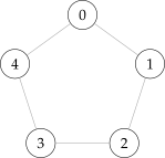
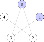
On a pair of $C_{5}$ confusion graphs, we want to define a graph product such that any neighboring $(i,j)$ brings overlaps on the decoding side. On a pair of $(u,v)$ and $(u^{\prime},v^{\prime})$ , they are adjacent iff

•

$u=u^{\prime}$ , $v$ and $v^{\prime}$ are adjacent on $C_{5}$ confusion graph;
•

$v=v^{\prime}$ , $u$ and $u^{\prime}$ are adjacent on $C_{5}$ confusion graph;
•

$u$ and $u^{\prime}$ , $v$ and $v^{\prime}$ are both adjacent on $C_{5}$ confusion graph.

We then define the symbol $\boxtimes$ such that $C_{5}\boxtimes C_{5}$ is illustrated as follows:

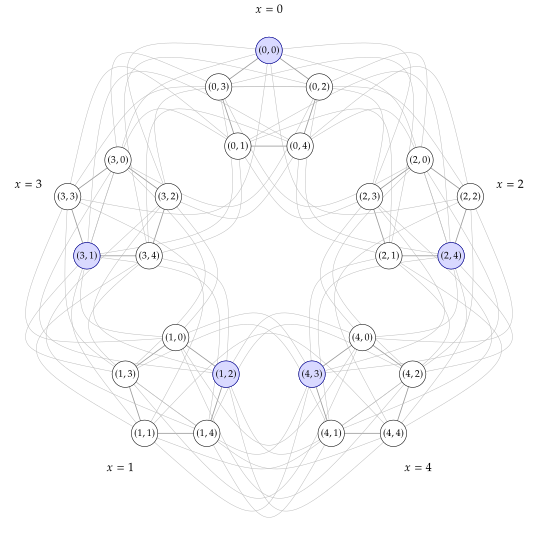
The new codewords form an independent set of size 5 on $C_{5}\boxtimes C_{5}$ , each $C_{5}$ is ordered as $0,2,4,1,3$ so that adjacency corresponds to difference $\pm 2\mod 5$ .

When it comes to general $(j,n)$ encoding and decoding functions, supposing it exists, then there must be $j\cdot 2^{n}\leq 5^{n}$ , such that for each of the $j$ values, the decoding boundary is $2^{n}$ , and the total area of decoding is no more than $5^{n}$ , or confusion must exists, and hence

n\geq\frac{\log_{2}j}{\log_{2}5-1}.

∎

Remark 1.10.48.

The 1.10.47 is the classical zero-error capacity viewpoint of Shannon [Sha56]. The pentagon case $C_{5}$ was solved by Lovász [Lov79].

Exercise 1.10.49 (Exercise 10.20 [MU17]).

A binary erasure channel transfers a sequences of $n$ bits. Each bit either arrives successfully without error or fails to arrive, and is replaced with a “?” symbol. Failure occur independently with probability $p$ . Define $(k,n)$ encoding and decoding functions for BEC similar to ones in the BSC, except that ${\mathsf{Dec}}:\{0,1,?\}^{n}\to\{0,1\}^{k}\cup\{\bot\}$ . Prove that, for any $p>0$ and any constants $\delta,\gamma>0$ , if $n$ is sufficiently large, then there exists $(k,n)$ encoding and decoding functions with $k\leq n(1-p-\delta)$ such that the probability that the receiver fails to obtain the correct message is at most $\gamma$ for every possible $k$ -bit message.

Proof.

The proof architecture is similar to lemmas 1.10.45 and 1.10.46, with a same setup of the randomized codewords, and the same encoding function. The decoder finds a codeword that has within $\left[\left\lceil n(p-\varepsilon)\right\rceil,\left\lfloor n(p+\varepsilon)% \right\rfloor\right]$ number of “?”, and the other symbols must match. If there is one such codeword, output the corresponding message; otherwise, reject by $\bot$ .

We reuse a few notations in lemma 1.10.45: Applying Hamming weight $\Delta$ over $\mathbf{x}_{i}\in\{0,1\}^{n}$ and $\mathbf{s}_{i}\leftarrow\mathbf{x}_{i}\oplus\mathbf{r}_{i}$ where $\mathbf{r}_{i}\in\{0,?\}^{n}$ , and $\oplus$ overrides $?$ to a symbol in $\{0,1\}$ . Then the weight defined in between $\mathbf{x}_{i}$ and $\mathbf{s}_{i}$ is

w(\mathbf{x}_{i},\mathbf{s}_{i})=p^{\Delta(\mathbf{x}_{i},\mathbf{s}_{i})}% \cdot(1-p)^{n-\Delta(\mathbf{x}_{i},\mathbf{s}_{i})}.

Let $\{S_{i}\}_{i\in[0,2^{k}-1]}$ be the set of $\{0,1,?\}^{n}$ decodable to $X_{i}$ , $\{W_{i}\}_{i\in[0,2^{k}-1]}$ be the set of probabilities that $X_{i}$ fails in decoding correctly, where

W_{i}=\sum_{\mathbf{r}\in\{0,?\}^{n},X_{i}\oplus\mathbf{r}\notin S_{i}}w(X_{i}% ,X_{i}\oplus\mathbf{r}).

It can also be expressed in the way that, let $1_{i,\mathbf{r}}$ be an indicator 0/1 random variable that is $1$ iff $X_{i}\oplus\mathbf{r}\notin S_{i}$ , then

W_{i}=\sum_{\mathbf{r}\in\{0,?\}^{n}}1_{i,\mathbf{r}}\cdot w(X_{i},X_{i}\oplus% \mathbf{r})=\sum_{\mathbf{r}\in T_{1}}1_{i,\mathbf{r}}\cdot w(X_{i},X_{i}% \oplus\mathbf{r})+\sum_{\mathbf{r}\in T_{2}}1_{i,\mathbf{r}}\cdot w(X_{i},X_{i% }\oplus\mathbf{r}),

by letting $T_{1}=\{\mathbf{r}\in\{0,?\}^{n}~{}:~{}\left|\Delta(\boldsymbol{0},\mathbf{r})% -np\right|>n\varepsilon\}$ and $T_{2}=\{\mathbf{r}\in\{0,?\}^{n}~{}:~{}\left|\Delta(\boldsymbol{0},\mathbf{r})% -np\right|\leq n\varepsilon\}$ .

WLOG we analyze $X_{0}$ , as by symmetry the same analysis hold for all other $X_{i}$ .

The first term is bounded in the same way as eq. 1.14 via Chernoff’s bound. Let $\{Z_{i}\}_{i\in[1,n]}$ be the independent Bernoulli trials with success probability $p$ , then $Z=\sum_{i\in[1,n]}Z_{i}$ is the number “?”s, for $0<\varepsilon<p$ ,

\sum_{\mathbf{r}\in T_{1}}1_{0,\mathbf{r}}\cdot w(X_{0},X_{0}\oplus\mathbf{r})% =\sum_{\mathbf{r}\in T_{1}}w(X_{0},X_{0}\oplus\mathbf{r})=\Pr\left[\left|Z-np% \right|>n\varepsilon\right]\leq\left(\frac{e^{\theta}}{(1+\theta)^{1+\theta}}% \right)^{np}+\left(\frac{e^{-\theta}}{(1-\theta)^{1-\theta}}\right)^{np}\leq 2% \exp\left(-\frac{\mu\theta^{2}}{3}\right),

For any threshold $0<\varepsilon<p$ , there is $n$ sufficiently large such that $2\exp\left(-\mu\theta^{2}/3\right)\leq\gamma/2$ .

It suffices to argue with respect to $X_{0}=\boldsymbol{0}$ for the second term by the same symmetry discussed in lemma 1.10.45, then the random variable

\sum_{\mathbf{r}\in T_{2}}1_{0,\mathbf{r}}\cdot w(\boldsymbol{0},\mathbf{r})

is dependent on $\{X_{i}\}_{i\in[1,2^{k}-1]}$ . For $\mathbf{r}\in T_{2}$ , averaging over $\{X_{i}\}_{i\in[1,2^{k}-1]}$ ,

\operatorname*{\mathbb{E}}\left[1_{0,\mathbf{r}}\cdot w(\boldsymbol{0},\mathbf% {r})\right]=w(\boldsymbol{0},\mathbf{r})\cdot\Pr\left[\exists i\in[1,2^{k}-1],% \left|\Delta(X_{i},\mathbf{r})-np\right|\leq n\varepsilon\right].

Supposing we have

\Pr\left[\exists i\in[1,2^{k}-1],\left|\Delta(X_{i},\mathbf{r})-np\right|\leq n% \varepsilon\right]\leq\frac{\gamma}{2},

then the second term can be upper bounded by

\sum_{\mathbf{r}\in T_{2}}\operatorname*{\mathbb{E}}\left[1_{0,\mathbf{r}}% \cdot w(\boldsymbol{0},\mathbf{r})\right]\leq\sum_{\mathbf{r}\in T_{2}}w(% \boldsymbol{0},\mathbf{r})\cdot\frac{\gamma}{2}\leq\frac{\gamma}{2}.

We continue by upper bounding the number of possible $n$ bits to derive $\mathbf{r}$ by $2^{\Delta(\boldsymbol{0},\mathbf{r})}\leq 2^{n(p+\varepsilon)}$ , then the probability of a particular codeword $X_{i}$ with $i>0$ being able to produce $\mathbf{r}$ is at most $2^{n(p+\varepsilon-1)}$ . Union bounding over all other codewords, the probability of other codeword failing decoding $\boldsymbol{0}$ is upper bounded by

(2^{k}-1)\cdot 2^{n(p+\varepsilon-1)}\leq 2^{k}\cdot 2^{n(p+\varepsilon-1)}% \leq 2^{n(\varepsilon-\delta)},

where the last inequality is by $k\leq n(1-p-\delta)$ . Since $2^{n(\varepsilon-\delta)}\to 0$ as $n\to\infty$ if $\delta>\varepsilon$ , then it is at most $\gamma/2$ on an $n$ . By symmetry, we conclude

\sum_{\mathbf{r}\in T_{2}}\operatorname*{\mathbb{E}}\left[1_{0,\mathbf{r}}% \cdot w(X_{0},X_{0}\oplus\mathbf{r})\right]\leq\frac{\gamma}{2}.

Combining the separated cases, we have

\operatorname*{\mathbb{E}}\left[W_{0}\right]=\sum_{\mathbf{r}\in T_{1}}% \operatorname*{\mathbb{E}}\left[1_{0,\mathbf{r}}\cdot w(X_{0},X_{0}\oplus% \mathbf{r})\right]+\sum_{\mathbf{r}\in T_{2}}\operatorname*{\mathbb{E}}\left[1% _{0,\mathbf{r}}\cdot w(X_{0},X_{0}\oplus\mathbf{r})\right]\leq\gamma.

By symmetry and linearity of expectation,

\sum_{i\in[0,2^{k}-1]}\operatorname*{\mathbb{E}}\left[W_{i}\right]\leq 2^{k}\gamma.

By the same ranking argument in theorem 1.10.46, there exists a set of codewords with at least $2^{k-1}$ codewords with $W_{i}\leq 2\gamma$ , and we choose the half of the set of codewords with small $W_{i}$ , and we complete the proof. ∎

Exercise 1.10.50 (Exercise 10.21 [MU17]).

In lemmas 1.10.45 and 1.10.46, we let decoder find a codeword with Hamming distance to the bits received within $\left[n(p-\varepsilon),n(p+\varepsilon)\right]$ . Instead, let decoder find the codeword by looking for the codeword with least number of differences, and break ties arbitrarily. Show how to modify the proof for lemmas 1.10.45 and 1.10.46 to obtain a similar result.

Proof.

Just use the Hamming ball of radius $\left\lfloor n(p+\varepsilon)\right\rfloor$ around the codeword. The “too far” Chernoff case still decays exponentionally fast, and the “in radius” case should approach 0 as $n\to\infty$ . ∎

	$\displaystyle\binom{n}{nq_{1};\ldots;nq_{6}}$	$\displaystyle\geq\frac{2^{nH(q_{1},\ldots,q_{6})}\cdot\left\|I\right\|^{\left\|I% \right\|/2}}{\left(2\pi n\right)^{(\left\|I\right\|-1)/2}}\cdot\prod_{i\in I}\exp% \left(-\frac{1}{12nq_{i}}\right)$
		$\displaystyle\geq\frac{2^{nH(q_{1},\ldots,q_{6})}\cdot\left\|I\right\|^{\left\|I% \right\|/2}}{\left(2\pi n\right)^{(\left\|I\right\|-1)/2}}\cdot\exp\left(-\frac{% \left\|I\right\|}{12}\right)$
		$\displaystyle=\frac{2^{nH(q_{1},\ldots,q_{6})}}{n^{(\left\|I\right\|-1)/2}}\cdot% \sqrt{2\pi}\cdot\left(\frac{\left\|I\right\|}{2\pi\exp\left(1/6\right)}\right)^{% \left\|I\right\|/2},$