1 Probability and Computing 1.12 Coupling of Markov Chains 1.14 Sample Complexity, VC Dimension, and Rademacher Complexity

1.13 Martingales

1.13.1 Martingales

Definition 1.13.1 (Martingale).

A sequence of random variables $Z_{0},Z_{1},\ldots$ is a martingale with respect to another sequence $X_{0},X_{1},\ldots$ if for all $n\geq 0$ , the following conditions hold:

•

$Z_{n}$ is a function of $X_{0},\ldots,X_{n}$ .
•

$\operatorname*{\mathbb{E}}\left[\left|Z_{n}\right|\right]<\infty$ .
•

$\operatorname*{\mathbb{E}}\left[Z_{n+1}\mid X_{0},\ldots,X_{n}\right]=Z_{n}$ .

A sequence of random variables $Z_{0},Z_{1},\ldots$ is called a martingale when it is a martingale with respect to itself, that is

•

$\operatorname*{\mathbb{E}}\left[\left|Z_{n}\right|\right]<\infty$ .
•

$\operatorname*{\mathbb{E}}\left[Z_{n+1}\mid Z_{0},\ldots,Z_{n}\right]=Z_{n}$ .

Example 1.13.2 (Martingale from Fair Games).

Consider a gambler who plays a sequence of fair games. Let $X_{i}$ be the winning on the $i^{\mathrm{th}}$ game, that is either $+1$ or $-1$ , and $Z_{i}$ be the gambler’s total winning of the first $i$ games. Since $Z_{0}=0$ and

Z_{i}=Z_{0}+\sum_{j\in[1,i]}X_{j},

then by linearity of expectation,

\operatorname*{\mathbb{E}}\left[Z_{i+1}\mid X_{1},\ldots,X_{i}\right]=Z_{i}+% \operatorname*{\mathbb{E}}\left[X_{i+1}\mid X_{1},\ldots,X_{i}\right]=Z_{i},

where the second equality holds as $\operatorname*{\mathbb{E}}\left[X_{i+1}\mid X_{1},\ldots,X_{i}\right]=0$ on any input of $X_{1},\ldots,X_{i}$ by fair game.

Thus, $Z_{1},\ldots,Z_{n}$ is a martingale with respect to the sequence $X_{1},\ldots,X_{n}$ .

Exercise 1.13.3 (Exercise 13.2 [MU17]).

Let $X_{0},X_{1},\ldots$ be a sequence of random variables, and let $S_{i}=\sum_{j\in[1,i]}X_{j}$ . Show that $S_{0},S_{1},\ldots$ is a martingale with respect to $X_{0},X_{1},\ldots$ , then for all $i\neq j$ , $\operatorname*{\mathbb{E}}\left[X_{i}X_{j}\right]=0$ .

Proof.

If $S_{0},S_{1},\ldots$ is a martingale with respect to $X_{0},X_{1},\ldots$ , then by definition 1.13.1,

S_{i}=\operatorname*{\mathbb{E}}\left[S_{i+1}\mid X_{0},\ldots,X_{i}\right]=S_% {i}+\operatorname*{\mathbb{E}}\left[X_{i+1}\mid X_{0},\ldots,X_{i}\right],

where the second equality holds by linearity of expectation, then for all $i\geq 0$ ,

\operatorname*{\mathbb{E}}\left[X_{i+1}\mid X_{0},\ldots,X_{i}\right]=0.

Hence, on an $i\geq 1$ and any $j<i$ , conditioned that $X_{j}=x$ ,

\operatorname*{\mathbb{E}}\left[X_{i}\mid X_{j}=x\right]=\operatorname*{% \mathbb{E}}\left[\operatorname*{\mathbb{E}}\left[X_{i}\mid X_{0},\ldots,X_{j}=% x,\ldots,X_{i-1}\right]\right]=0.

Therefore, we conclude the proof by

	$\displaystyle\operatorname*{\mathbb{E}}\left[X_{i}X_{j}\right]$	$\displaystyle=\operatorname{\mathbb{E}}\left[\operatorname{\mathbb{E}}\left[% X_{i}X_{j}\mid X_{j}\right]\right]$
		$\displaystyle=\sum_{x\in\Omega}\operatorname*{\mathbb{E}}\left[X_{i}X_{j}\mid X% _{j}=x\right]\Pr\left[X_{j}=x\right]$
		$\displaystyle=\sum_{x\in\Omega}x\operatorname*{\mathbb{E}}\left[X_{i}\mid X_{j% }=x\right]\Pr\left[X_{j}=x\right]=0.$

∎

Exercise 1.13.4 (Exercise 13.1 [MU17]).

Show that if $Z_{0},Z_{1},\ldots$ is a martingale with respect to $X_{0},X_{1},\ldots$ , then it is a martingale with respect to itself.

Proof.

By definition 1.2.6 and lemma 1.2.7, we use the tower property

\operatorname*{\mathbb{E}}\left[\operatorname*{\mathbb{E}}\left[Y\mid X\right]% \mid Z\right]=\operatorname*{\mathbb{E}}\left[Y\mid Z\right]

for random variables $X, Y, Z$ such that $Z$ is determined by $X$ , or $X$ carries at least as much information as $Z$ , or $Z$ can be obtained from $X$ from some function.

Since $Z_{0},\ldots,Z_{n}$ is a martingale with respect to $X_{0},\ldots,X_{n}$ , then by definition 1.13.1, for all $i\in[0,n]$ ,

Z_{i}=\operatorname*{\mathbb{E}}\left[Z_{i+1}\mid X_{0},\ldots,X_{i}\right].

By the prior fact,

\operatorname*{\mathbb{E}}\left[\operatorname*{\mathbb{E}}\left[Z_{i+1}\mid X_% {0},\ldots,X_{i}\right]\mid Z_{0},\ldots,Z_{i}\right]=\operatorname*{\mathbb{E% }}\left[Z_{i+1}\mid Z_{0},\ldots,Z_{i}\right].

Yet by definition 1.13.1,

\operatorname*{\mathbb{E}}\left[\operatorname*{\mathbb{E}}\left[Z_{i+1}\mid X_% {0},\ldots,X_{i}\right]\mid Z_{0},\ldots,Z_{i}\right]=\operatorname*{\mathbb{E% }}\left[Z_{i}\mid Z_{0},\ldots,Z_{i}\right]=Z_{i}.

Therefore we conclude by $\operatorname*{\mathbb{E}}\left[Z_{i+1}\mid Z_{0},\ldots,Z_{i}\right]=Z_{i}$ . ∎

Exercise 1.13.5 (Exercise 13.4 [MU17]).

Let $X_{1},X_{2},\ldots$ be independent identically distributed random variables with expectation 0 and variance $\sigma^{2}<\infty$ . Let

Z_{n}=\left(\sum_{i\in[1,n]}X_{i}\right)^{2}-n\sigma^{2}.

Show that $Z_{1},Z_{2},\ldots$ is a martingale.

Proof.

Let $Y_{n}=\sum_{i\in[1,n]}X_{i}$ , then $Z_{n}=Y_{n}^{2}-n\sigma^{2}$ . Since $\operatorname*{\mathbb{E}}\left[X_{i}\right]=0$ , then $\sigma^{2}=\operatorname*{\mathbb{E}}\left[X_{i}^{2}\right]$ . We show as follows: For $n\geq 1$ ,

	$\displaystyle\operatorname*{\mathbb{E}}\left[Z_{n+1}\mid X_{1},\ldots,X_{n}\right]$	$\displaystyle=\operatorname*{\mathbb{E}}\left[Z_{n}+X_{n+1}^{2}+2X_{n+1}Y_{n}-% \sigma^{2}\mid X_{1},\ldots,X_{n}\right]$
		$\displaystyle=Z_{n}+\operatorname{\mathbb{E}}\left[X_{n+1}^{2}\right]+2% \operatorname{\mathbb{E}}\left[X_{n+1}Y_{n}\right]-\sigma^{2}$
		$\displaystyle=Z_{n}+\operatorname{\mathbb{E}}\left[X_{n+1}^{2}\right]+2% \operatorname{\mathbb{E}}\left[X_{n+1}\right]\operatorname*{\mathbb{E}}\left[% Y_{n}\right]-\sigma^{2}$
		$\displaystyle=Z_{n}+\operatorname*{\mathbb{E}}\left[X_{n+1}^{2}\right]-\sigma^% {2}=Z_{n},$

where the second and the third equality are from the independence, and the last two equalities are from expectation being 0. By 1.13.4, we conclude the proof. ∎

Definition 1.13.6 (Doob Martingale [Doo40]).

Let $X_{0},\ldots,X_{n}$ be a sequence of random variables, and $Y$ be a random variable depending on $X_{0},\ldots,X_{n}$ with $\operatorname*{\mathbb{E}}\left[\left|Y\right|\right]<\infty$ , then for $i\in[0,n]$ ,

Z_{i}=\operatorname*{\mathbb{E}}\left[Y\mid X_{0},\ldots,X_{i}\right]

gives a martingale with respect to $X_{0},\ldots,X_{n}$ , as

	$\displaystyle\operatorname*{\mathbb{E}}\left[Z_{i+1}\mid X_{0},\ldots,X_{i}\right]$	$\displaystyle=\operatorname{\mathbb{E}}\left[\operatorname{\mathbb{E}}\left[% Y\mid X_{0},\ldots,X_{i+1}\right]\mid X_{0},\ldots,X_{i}\right]$
		$\displaystyle=\operatorname*{\mathbb{E}}\left[Y\mid X_{0},\ldots,X_{i}\right]$
		$\displaystyle=Z_{i},$

where the second equality holds by lemma 1.2.7 and definition 1.2.6.

Remark 1.13.7.

One can view the Doob Martingale as a sequence of refined predictions to $Y$ , where each element $Z_{i}$ is the expectation of $Y$ when the values of $X_{0},\ldots,X_{i}$ are known. Hence, the refined predictions gradually using more information on the values of the random variables $X_{0},\ldots,X_{n}$ .

Exercise 1.13.8 (Exercise 13.3 [MU17]).

Let $X_{0}=0$ and for $j\geq 0$ , $X_{j+1}$ is chosen uniformly over real interval $[X_{j},1]$ . Show that, for $k\geq 0$ , the sequence $Y_{k}=2^{k}(1-X_{k})$ is a martingale.

Proof.

Since $Y_{k+1}$ depends only on $Y_{k}$ , then

\operatorname*{\mathbb{E}}\left[Y_{k+1}\mid Y_{0},\ldots,Y_{k}\right]=% \operatorname*{\mathbb{E}}\left[Y_{k+1}\mid Y_{k}\right].

Moreover, since $\operatorname*{\mathbb{E}}\left[X_{k+1}\mid X_{k}\right]=(1+X_{k})/2$ , then

\operatorname*{\mathbb{E}}\left[Y_{k+1}\mid X_{k}\right]=\operatorname*{% \mathbb{E}}\left[2^{k+1}(1-X_{k+1})\mid X_{k}\right]=2^{k+1}-2^{k+1}% \operatorname*{\mathbb{E}}\left[X_{k+1}\mid X_{k}\right]=2^{k}(1-X_{k})=Y_{k}.

By $\operatorname*{\mathbb{E}}\left[Y_{k}\mid Y_{k}\right]=Y_{k}$ , we show that

\operatorname*{\mathbb{E}}\left[\operatorname*{\mathbb{E}}\left[Y_{k+1}\mid X_% {k}\right]\mid Y_{k}\right]=\operatorname*{\mathbb{E}}\left[Y_{k+1}\mid Y_{k}% \right]=Y_{k},

which concludes the proof. ∎

Lemma 1.13.9.

If $Z_{0},Z_{1},\ldots$ is a martingale with respect to $X_{0},X_{1},\ldots$ , then $\operatorname*{\mathbb{E}}\left[Z_{n}\right]=\operatorname*{\mathbb{E}}\left[Z% _{0}\right]$ for any $n\geq 0$ .

Proof.

By definition 1.13.1, for any $n\geq 1$

\operatorname*{\mathbb{E}}\left[Z_{n}\mid X_{0},\ldots,X_{n-1}\right]=Z_{n-1}.

Given that

\operatorname*{\mathbb{E}}\left[Z_{n-1}\mid X_{0},\ldots,X_{n-2}\right]=Z_{n-2},

we have

	$\displaystyle Z_{n-2}$	$\displaystyle=\operatorname*{\mathbb{E}}\left[Z_{n-1}\mid X_{0},\ldots,X_{n-2}\right]$
		$\displaystyle=\operatorname{\mathbb{E}}\left[\operatorname{\mathbb{E}}\left[% Z_{n}\mid X_{0},\ldots,X_{n-1}\right]\mid X_{0},\ldots,X_{n-2}\right]$
		$\displaystyle=\operatorname*{\mathbb{E}}\left[Z_{n}\mid X_{0},\ldots,X_{n-2}% \right].$

By induction, we have $Z_{0}=\operatorname*{\mathbb{E}}\left[Z_{n}\mid X_{0}\right]$ , then

\operatorname*{\mathbb{E}}\left[Z_{0}\right]=\operatorname*{\mathbb{E}}\left[% \operatorname*{\mathbb{E}}\left[Z_{n}\mid X_{0}\right]\right]=\operatorname*{% \mathbb{E}}\left[Z_{n}\right],

which concludes the proof. ∎

Example 1.13.10 (Galton-Watson Process).

The Galton-Watson process was used in theorem 1.6.60, but was originally used to statistically investigate the extinction of family names. Let $G_{t}$ be the random variable for the individuals in the $t^{\mathrm{th}}$ generation, and $X_{t,k}$ be the number of offspring of the $k^{\mathrm{th}}$ individual in the $t^{\mathrm{th}}$ generation. Each individual gives birth to offspring independently, and their numbers of offspring are identically distributed. Hence,

G_{t}=\sum_{k\in[1,G_{t-1}]}X_{t-1,k},

and let $\mu=\operatorname*{\mathbb{E}}\left[X_{t,k}\right]$ . By linearity of expectation,

\operatorname*{\mathbb{E}}\left[G_{t+1}\mid G_{1},\ldots,G_{t}\right]=\mu G_{t}.

Let $M_{t}=\mu^{-t}\cdot G_{t}$ , then

\operatorname*{\mathbb{E}}\left[M_{t+1}\mid G_{1},\ldots,G_{t}\right]=% \operatorname*{\mathbb{E}}\left[\mu^{-(t+1)}\cdot G_{t+1}\mid G_{1},\ldots,G_{% t}\right]=\mu^{-t}\cdot G_{t}=M_{t},

and we have

\operatorname*{\mathbb{E}}\left[\operatorname*{\mathbb{E}}\left[M_{t+1}\mid G_% {1},\ldots,G_{t}\right]\mid M_{1},\ldots,M_{t}\right]=\operatorname*{\mathbb{E% }}\left[M_{t+1}\mid M_{1},\ldots,M_{t}\right].

On the other hand,

\operatorname*{\mathbb{E}}\left[\operatorname*{\mathbb{E}}\left[M_{t+1}\mid G_% {1},\ldots,G_{t}\right]\mid M_{1},\ldots,M_{t}\right]=\operatorname*{\mathbb{E% }}\left[M_{t}\mid M_{1},\ldots,M_{t}\right]=M_{t},

which makes $M_{1},\ldots$ a martingale.

Example 1.13.11 (Pólya’s Urn).

Suppose there are black balls and white balls in an urn, that are identical except for the colors. Each time pick a ball, and put it back with another identical ball with same color. For simplicity, we start at round 2, and ends at round $n$ where there are $n$ balls in the urn. Let $X_{n}$ be the number of black balls in the urn, and $Z_{n}=X_{n}/n$ be the ratio of black balls in the urn. Then for all $n\geq 2$ ,

\operatorname*{\mathbb{E}}\left[Z_{n+1}\mid Z_{2},\ldots,Z_{n}\right]=Z_{n}% \cdot\frac{nZ_{n}+1}{n+1}+(1-Z_{n})\cdot\frac{nZ_{n}}{n+1}=Z_{n},

which makes $Z_{2},Z_{3},\ldots$ a martingale.

1.13.2 Stopping Times

By lemma 1.13.9, if the number of games is fixed initially, then the expected gain from the fair games is $0$ , if $Z_{0}=0$ . But suppose the number of games is not fixed initially, for example the gambler choose to play a random number of games, by deciding when to quit based on the outcome of the games already played.

Definition 1.13.12 (Stopping Time).

A nonnegative integer-valued random variable $T$ is a stopping time for the sequence $Z_{0},Z_{1},\ldots$ if the probability of the event $T=n$ is independent of the variables $\{Z_{n+j}\mid Z_{0},\ldots,Z_{n}\}_{j\geq 1}$ , which are the random variables $Z_{n+1},Z_{n+2},\ldots$ conditioned on the values of $Z_{0},\ldots,Z_{n}$ .

A stopping time is corresponding to a strategy of when to stop based only on the outcome seen so far. But given that one can stop by strategy such as “winning reaches 10 for the first time”, it would be helpful to characterize the conditions on the stopping time $T$ that maintain the property $\operatorname*{\mathbb{E}}\left[Z_{T}\right]=\operatorname*{\mathbb{E}}\left[Z% _{0}\right]=0$ . The subtle problem is that, $T$ might not be finite in this case, that the gambler will gamble infinite number of times with non-zero probability. The martingale stopping time theorem shows that, under certain conditions, and in particular when the stopping time is bounded or has bounded expectation, the expected value of the martingale at the stopping time is $\operatorname*{\mathbb{E}}\left[Z_{0}\right]$ .

Theorem 1.13.13 (Martingale Stopping Time Theorem).

If $Z_{0},Z_{1},\ldots$ is a martingale with respect to $X_{0},X_{1},\ldots$ and if $T$ is a stopping time for $X_{0},X_{1},\ldots$ , then

\operatorname*{\mathbb{E}}\left[Z_{T}\right]=\operatorname*{\mathbb{E}}\left[Z% _{0}\right]

whenever one of the following holds:

•

The $Z_{i}$ is bounded, such that there exists constant $c$ for all $i\geq 0$ , $\left|Z_{i}\right|\leq c$ .
•

$T$ is bounded.
•

$\operatorname*{\mathbb{E}}\left[T\right]<\infty$ , and there is a constant $c$ such that $\operatorname*{\mathbb{E}}\left[\left|Z_{i+1}-Z_{i}\right|\mid X_{0},\ldots,X_% {i}\right]\leq c$ .

Exercise 1.13.14 (Exercise 13.5 [MU17]).

Consider the gambler’s ruin example 1.7.51, stopping by either losing $\ell_{1}$ or winning $\ell_{2}$ . Let $X_{n}$ be the winning in the $n^{\mathrm{th}}$ game, $Y_{n}$ be the winning by the end of the $n^{\mathrm{th}}$ game, and $Z_{n}=Y_{n}^{2}-n$ . Show that $Z_{1},Z_{2},\ldots$ is a martingale, and let $T$ be a stopping time, determine $\operatorname*{\mathbb{E}}\left[Z_{T}\right]$ and $\operatorname*{\mathbb{E}}\left[T\right]$ .

Proof.

Since $\mathrm{Var}\left[X_{i}\right]=1$ and $\operatorname*{\mathbb{E}}\left[X_{i}\right]=0$ , by 1.13.5, $Z_{1},Z_{2},\ldots$ is a martingale.

We have shown in 1.7.68 that $\operatorname*{\mathbb{E}}\left[T\right]=\ell_{1}\ell_{2}$ .

The theorem 1.13.13 applies by

\left|Z_{i+1}-Z_{i}\right|=\left|\left(Y_{i+1}-Y_{i}\right)\left(Y_{i+1}+Y_{i}% \right)-1\right|\leq\left|Y_{i+1}-Y_{i}\right|\cdot\left|Y_{i+1}+Y_{i}\right|+% 1\leq 2\max\left(\ell_{1},\ell_{2}\right)+1,

then $\operatorname*{\mathbb{E}}\left[Z_{T}\right]=\operatorname*{\mathbb{E}}\left[Z% _{1}\right]=0$ , which means $\operatorname*{\mathbb{E}}\left[Y_{T}^{2}\right]=\operatorname*{\mathbb{E}}% \left[T\right]$ . Since $Y_{T}^{2}$ can either be $\ell_{1}^{2}$ or $\ell_{2}^{2}$ , by example 1.7.51 ¹⁶¹⁶16 Now we can show by $Y_{i}$ is a martingale in example 1.13.2, then $\operatorname*{\mathbb{E}}\left[Y_{T}\right]=0$ , to derive the winning or losing probabilities. ,

\operatorname*{\mathbb{E}}\left[Y_{T}^{2}\right]=\ell_{1}^{2}\cdot\frac{\ell_{% 2}}{\ell_{1}+\ell_{2}}+\ell_{2}^{2}\cdot\frac{\ell_{1}}{\ell_{1}+\ell_{2}}=% \ell_{1}\ell_{2},

which derives $\operatorname*{\mathbb{E}}\left[T\right]$ in a martingale way. ∎

Exercise 1.13.15 (Exercise 13.6 [MU17]).

Consider the gambler’s ruin example 1.7.51, stopping by either losing $\ell_{1}$ or winning $\ell_{2}$ , and winning probability $p<1/2$ . Let $X_{n}$ be the winning in the $n^{\mathrm{th}}$ game, and $Z_{n}$ be the winning by the end of the $n^{\mathrm{th}}$ game.

•

Show that

$A_{n}=\left(\frac{1-p}{p}\right)^{Z_{n}}$

is a martingale with mean 1.
•

Determine the probability that the player wins $\ell_{2}$ before losing $\ell_{1}$ .
•

Show that $B_{n}=Z_{n}-(2p-1)n$ is a martingale with mean 0.
•

Let $T$ be the stopping time when the player finishes playing. Determine $\operatorname*{\mathbb{E}}\left[Z_{T}\right]$ and $\operatorname*{\mathbb{E}}\left[T\right]$ .

Proof.

We have shown in 1.7.69 that

A_{n}=\left(\frac{1-p}{p}\right)^{Z_{n}},

we have $\operatorname*{\mathbb{E}}\left[A_{n+1}\right]=\operatorname*{\mathbb{E}}\left% [A_{n}\right]=1$ . Since $Z_{n+1}=Z_{n}+X_{n+1}$ ,

\operatorname*{\mathbb{E}}\left[A_{n+1}\mid X_{1},\ldots,X_{n}\right]=p\left(% \frac{1-p}{p}\right)^{Z_{n}+1}+(1-p)\left(\frac{1-p}{p}\right)^{Z_{n}-1}=\left% (\frac{1-p}{p}\right)^{Z_{n}}=A_{n},

which proves that $A_{1},A_{2},\ldots$ is a martingale by 1.13.4.

With this $A_{1},A_{2},\ldots$ martingale, then let $q$ be the probability of being absorbed into $\ell_{2}$ , and

\operatorname*{\mathbb{E}}\left[A_{T}\right]=q\left(\frac{1-p}{p}\right)^{\ell% _{2}}+(1-q)\left(\frac{1-p}{p}\right)^{-\ell_{1}}=1,

such that

q=\left(1-\left(\frac{1-p}{p}\right)^{\ell_{1}}\right)\cdot\left(1-\left(\frac% {1-p}{p}\right)^{\ell_{1}+\ell_{2}}\right)^{-1}.

Since $\operatorname*{\mathbb{E}}\left[X_{i}\right]=p-(1-p)=2p-1$ , then by linearity of expectation,

\operatorname*{\mathbb{E}}\left[B_{n+1}\mid X_{1},\ldots,X_{n}\right]=B_{n}+% \operatorname*{\mathbb{E}}\left[X_{n+1}-(2p-1)\mid X_{1},\ldots,X_{n}\right]=B% _{n},

the second equality holds by the independence of the games. Hence, $B_{1},B_{2},\ldots$ is a martingale by 1.13.4.

Since $A_{n}$ is bounded, then by theorem 1.13.13, $\operatorname*{\mathbb{E}}\left[A_{T}\right]=\operatorname*{\mathbb{E}}\left[A% _{1}\right]=1$ . Therefore,

\operatorname*{\mathbb{E}}\left[Z_{T}\right]=-\ell_{1}\cdot(1-q)+\ell_{2}\cdot q% =(\ell_{1}+\ell_{2})\cdot q-\ell_{1}.

By $\operatorname*{\mathbb{E}}\left[B_{T}\right]=0=\operatorname*{\mathbb{E}}\left% [Z_{T}\right]-(2p-1)\operatorname*{\mathbb{E}}\left[T\right]$ , we have

\operatorname*{\mathbb{E}}\left[T\right]=\frac{\operatorname*{\mathbb{E}}\left% [Z_{T}\right]}{2p-1}=\frac{\ell_{1}-(\ell_{1}+\ell_{2})\cdot q}{1-2p}.

∎

Example 1.13.16 (A Ballot Theorem).

Suppose there are 2 candidates running an election, where candidate A obtains $a$ votes, and candidate B obtains $b<a$ votes. The votes come in random order, and can be viewed as sampled from uniformly random permutations. Candidate A always with higher votes has probability $(a-b)/(a+b)$ .

Let $n=a+b$ , and let $S_{k}$ be the leading votes of A to B after $k$ votes. Then $S_{n}=a-b$ . For $0\leq k\leq n-1$ , let

X_{k}=\frac{S_{n-k}}{n-k}.

We first show that $X_{1},X_{2},\ldots,X_{n}$ is a martingale. Since

\operatorname*{\mathbb{E}}\left[S_{n-k-1}\mid S_{n},\ldots,S_{n-k}\right]=% \operatorname*{\mathbb{E}}\left[S_{n-k-1}\mid S_{n-k}\right]=\frac{n-k+S_{n-k}% }{2(n-k)}\cdot(S_{n-k}-1)+\frac{n-k-S_{n-k}}{2(n-k)}\cdot(S_{n-k}+1)=\frac{n-k% -1}{n-k}\cdot S_{n-k},

where the first equality holds by $S_{n-k-1}$ is only related to $S_{n-k}$ counting backwards, and the second equality holds by the probability of the $(n-k)^{\mathrm{th}}$ vote being A or B, conditioned on $S_{n-k}$ , then

\operatorname*{\mathbb{E}}\left[X_{k+1}\mid S_{n},\ldots,S_{n-k}\right]=\frac{% S_{n-k}}{n-k}=X_{k},

and

\operatorname*{\mathbb{E}}\left[X_{k+1}\mid X_{1},\ldots,X_{k}\right]=% \operatorname*{\mathbb{E}}\left[\operatorname*{\mathbb{E}}\left[X_{k+1}\mid S_% {n},\ldots,S_{n-k}\right]\mid X_{1},\ldots,X_{k}\right]=X_{k},

which completes the proof of martingale.

Moreover, define a stopping $T$ for the first $X_{T}=0$ , otherwise $T=n-1$ , then since $T$ is bounded, and $X_{0},\ldots,X_{n-1}$ is also bounded, by theorem 1.13.13,

\operatorname*{\mathbb{E}}\left[X_{T}\right]=\operatorname*{\mathbb{E}}\left[X% _{0}\right]=\frac{S_{n}}{n}=\frac{a-b}{a+b}.

By the stopping time $T$ , the voting is either A and B are drawing, or A leads throughout the $n$ votes. In the first case, $X_{T}=0$ as $S_{T}=0$ , otherwise, $X_{T}=1$ as $S_{T}=n$ . Hence,

\operatorname*{\mathbb{E}}\left[X_{T}\right]=\Pr\left[\text{A leads throughout% }\right]\cdot 1+\Pr\left[\text{A and B are drawing}\right]\cdot 0=\frac{a-b}{a% +b},

which completes the proof.

Remark 1.13.17.

The example 1.13.16 is also called Bertrand’s ballot theorem, which can be proved in other ways.

One of the earliest proofs [And87] solved the problem directly, but the “geometric reflection” trick derives from his work. Consider a 2-dimensional lattice, a vote for A moves is a step right, and a vote for B is a step up. Hence, after $n$ moves, the particle moves from $(0,0)$ to $(a,b)$ . An observation is, if A is ahead in the count throughout, then the particle is constantly below the line $y=x$ (except for the initial state with no vote).

Moreover, for any permutation that start with a vote for B, then it has to be at the diagonal $y=x$ at least once. The reflection trick is: we can always reflect a trajectory above the diagonal to the symmetry one below the diagonal $y=x$ , such that the move is still a bad move, but the move is beginning with a vote for A to $(1,0)$ .

Since all the valid trajectories begin with a vote for A, we just exclude all the bad trajectories beginning with $(1,0)$ , and all such bad trajectories can be reflected to the trajectories beginning with $(0,1)$ .

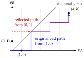
Therefore, the number of valid trajectories is

\binom{a+b-1}{a-1}-\binom{a+b-1}{b-1}=\frac{a-b}{a+b}\cdot\binom{a+b}{a}.

When $a=b+1$ , this deteriorates to lemma 1.7.67, which are Dycks path and Catalans number $C_{b}$ .

1.13.3 Wald’s Equation

Wald’s equation is an important corollary of theorem 1.13.13, which handles the expectation of the sum of independent random variables, where the number of random variables being summed is itself a random variable.

Theorem 1.13.18 (Wald’s Equation [Wal47]).

Let $X_{1},X_{2},\ldots$ be independent, identically distributed random variables with distribution $X$ , and $T$ be a stopping time for this sequence. If $T$ and $X$ have bounded expectation, then

\operatorname*{\mathbb{E}}\left[\sum_{i\in[1,T]}X_{i}\right]=\operatorname*{% \mathbb{E}}\left[T\right]\cdot\operatorname*{\mathbb{E}}\left[X\right].

Proof.

We first show a version for the nonnegative random variables. For $i\geq 1$ , let

Z_{i}=\sum_{j\in[1,i]}\left(X_{j}-\operatorname*{\mathbb{E}}\left[X_{j}\right]% \right),

then $Z_{1},Z_{2},\ldots$ is a martingale with respect to $X_{1},X_{2},\ldots$ , with $\operatorname*{\mathbb{E}}\left[Z_{i}\right]=0$ by 1.13.15.

Since $\operatorname*{\mathbb{E}}\left[T\right]<\infty$ , and

\operatorname*{\mathbb{E}}\left[\left|Z_{i+1}-Z_{i}\right|\mid X_{1},\ldots,X_% {i}\right]=\operatorname*{\mathbb{E}}\left[\left|X_{i+1}-\operatorname*{% \mathbb{E}}\left[X\right]\right|\right]\leq 2\operatorname*{\mathbb{E}}\left[X% \right],

(1.25)

then by theorem 1.13.13,

\operatorname*{\mathbb{E}}\left[Z_{T}\right]=\operatorname*{\mathbb{E}}\left[Z% _{1}\right]=0.

Therefore, by linearity of expectation,

\operatorname*{\mathbb{E}}\left[Z_{T}\right]=\operatorname*{\mathbb{E}}\left[% \sum_{i\in[1,T]}\left(X_{i}-\operatorname*{\mathbb{E}}\left[X\right]\right)% \right]=\operatorname*{\mathbb{E}}\left[\sum_{i\in[1,T]}X_{i}\right]-% \operatorname*{\mathbb{E}}\left[T\right]\cdot\operatorname*{\mathbb{E}}\left[X% \right],

which completes the proof.

In general case, where $X$ is any random variable, the main trick is writing $X=X^{+}-X^{-}$ , where

X^{+}=\max\left(X,0\right),\quad X^{-}=\max\left(-X,0\right).

Hence, write $X_{i}=X_{i}^{+}-X_{i}^{-}$ for all $i\geq 1$ , and by the prior nonnegative case,

\operatorname*{\mathbb{E}}\left[\sum_{i\in[1,T]}X_{i}^{+}\right]=\operatorname% *{\mathbb{E}}\left[T\right]\cdot\operatorname*{\mathbb{E}}\left[X^{+}\right],% \operatorname*{\mathbb{E}}\left[\sum_{i\in[1,T]}X_{i}^{-}\right]=\operatorname% *{\mathbb{E}}\left[T\right]\cdot\operatorname*{\mathbb{E}}\left[X^{-}\right].

By linearity of expectation,

	$\displaystyle\operatorname*{\mathbb{E}}\left[\sum_{i\in[1,T]}X_{i}\right]$	$\displaystyle=\operatorname{\mathbb{E}}\left[\sum_{i\in[1,T]}X_{i}^{+}-\sum_{% i\in[1,T]}X_{i}^{-}\right]=\operatorname{\mathbb{E}}\left[\sum_{i\in[1,T]}X_{% i}^{+}\right]-\operatorname*{\mathbb{E}}\left[\sum_{i\in[1,T]}X_{i}^{-}\right]$
		$\displaystyle=\operatorname{\mathbb{E}}\left[T\right]\cdot\left(\operatorname% {\mathbb{E}}\left[X^{+}\right]-\operatorname*{\mathbb{E}}\left[X^{-}\right]\right)$
		$\displaystyle=\operatorname{\mathbb{E}}\left[T\right]\cdot\operatorname{% \mathbb{E}}\left[X\right],$

we conclude the proof for the general case. ∎

Remark 1.13.19.

Since $T$ is a stopping time for $X_{1},X_{2},\ldots$ , then event $\{T\geq i\}$ is dependent only on $X_{1},\ldots,X_{i-1}$ by definition 1.13.12. The mutual independence over $X_{i}$ ensures that $X_{i}$ is independent of past $X_{1},\ldots,X_{i-1}$ , hence $X_{i}$ is independent of $\{T\geq i\}$ . The independence is a convenient sufficient condition, that can be used to construct martingale in 1.13.15 and used here, and help simplify the third condition of the theorem 1.13.13 in eq. 1.25.

After theorems 1.13.18, 1.13.19 and 1.13.15, for the stopping time in the case of independent random variables, we have an equivalent, yet simpler version of stopping time as follows.

Definition 1.13.20 (Stopping Time for Independent Random Variables).

Let $Z_{0},Z_{1},\ldots$ be a sequence of independent random variables. A nonnegative, integer-valued random variable $T$ is a stopping time for the sequence if the event $\{T=n\}$ is independent of $Z_{n+1},Z_{n+2},\ldots$ .

Example 1.13.21 (Dice Rolling).

Consider a gambling game where a player first rolls a die. If the outcome is $X$ then roll $X$ new standard dice and gain $Z$ , which is the sum of the outcome of the $X$ dice. This is exactly an application of theorem 1.13.18 to derive the expected outcome. By definition 1.13.20 and theorem 1.13.18, let $X$ be the stopping time, and $Y_{1},Y_{2},\ldots$ be i.i.d. random variables for dice rolling scores with distribution $Y$ . Then by theorem 1.13.18,

\operatorname*{\mathbb{E}}\left[\sum_{i\in[1,X]}Y_{i}\right]=\operatorname*{% \mathbb{E}}\left[X\right]\cdot\operatorname*{\mathbb{E}}\left[Y\right]=\left(% \frac{1+n}{2}\right)^{2},

if the die is a $n$ faced fair die.

Example 1.13.22 (Server Message Transmission).

Consider $n$ servers communicating using a shared channel, where time is divided in discrete slots. At each time slot, any server that needs to send a packet can transmit it through the channel. If exactly one packet is sent at that time, the transmission is successful, otherwise none are successful. At a time slot, a server transmits a packet with probability $1/n$ .

Let $X_{1},X_{2},\ldots$ be the independent 0-1 random variables for a successful packet transmission on the $i^{\mathrm{th}}$ time slot with distribution $X$ , then

\Pr\left[X=1\right]=\binom{n}{1}\cdot\frac{1}{n}\cdot\left(1-\frac{1}{n}\right% )^{n-1}=\left(1-\frac{1}{n}\right)^{n-1}.

Similar to section 1.5.1, let

\varphi_{g}(n)=(n-1)\ln\left(1-\frac{1}{n}\right),

then

\varphi_{g}^{\prime}(n)=\ln\left(1-\frac{1}{n}\right)+\frac{1}{n}.

Let $t=1-1/n$ , and $n\geq 2$ means $1/2\leq t<1$ , then $\varphi_{g}^{\prime}(n)<0$ . Therefore, when $n\geq 2$ , since

\lim_{n\to\infty}\left(1-\frac{1}{n}\right)^{n-1}=e^{-1},

then $e^{-1}$ is a lower bound by

p=\Pr\left[X=1\right]=\left(1-\frac{1}{n}\right)^{n-1}\geq e^{-1}.

Let $N$ be the random variable for the number of packets successfully sent until each server has successfully sent at least 1 packet. By the Coupon’s Collector’s Problem,

\operatorname*{\mathbb{E}}\left[N\right]=n\sum_{i\in[1,n]}i^{-1}=nH(n)=n\ln n+cn.

Let $Y_{i}$ be the number of time slots between the $(i-1)^{\mathrm{th}}$ successful transmission and the $i^{\mathrm{th}}$ successful transmission. Then $Y_{1},Y_{2},\ldots$ are independent and geometrically distributed with success probability $p$ , therefore $\operatorname*{\mathbb{E}}\left[Y_{i}\right]=1/p\leq e$ . Moreover, whichever server successfully transmitted a packet is independent of the waiting times $Y_{i}$ , so the Wald argument applies to this sum. By theorem 1.13.18,

\operatorname*{\mathbb{E}}\left[\sum_{i\in[1,N]}Y_{i}\right]=\operatorname*{% \mathbb{E}}\left[N\right]\cdot\operatorname*{\mathbb{E}}\left[Y_{1}\right]\leq e% \left(n\ln n+cn\right).

Exercise 1.13.23 (Exercise 13.11 [MU17]).

A parking-lot attendant has mixed up $n$ keys for $n$ cars. The $n$ car owners arrive together. The attendant gives each owner a key according to a permutation chosen uniformly at random from all permutations. If an owner receives his key, he takes it and leaves; otherwise, he returns the key to the attendant. The attendant repeats the process with the remaining keys and car owners. This continues until all owners receive the keys to their cars. Let $R$ be the number of rounds until all car owners receive their keys, and let $X_{i}$ be the number of owners who receive their car keys in the $i^{\mathrm{th}}$ round. Show that

Y_{i}=\sum_{j\in[1,i]}\left(X_{j}-\operatorname*{\mathbb{E}}\left[X_{j}\mid X_% {1},\ldots,X_{j-1}\right]\right)

is a martingale, and use theorem 1.13.13 to derive $\operatorname*{\mathbb{E}}\left[R\right]$ .

Proof.

To show that $Y_{1},Y_{2},\ldots$ is a martingale, we have

	$\displaystyle\operatorname*{\mathbb{E}}\left[Y_{i}\mid Y_{1},\ldots,Y_{i-1}\right]$	$\displaystyle=Y_{i-1}+\operatorname{\mathbb{E}}\left[X_{i}-\operatorname{% \mathbb{E}}\left[X_{i}\mid X_{1},\ldots,X_{i-1}\right]\mid Y_{1},\ldots,Y_{i-1% }\right]$
		$\displaystyle=Y_{i-1}+\operatorname{\mathbb{E}}\left[X_{i}\mid Y_{1},\ldots,Y% _{i-1}\right]-\operatorname{\mathbb{E}}\left[X_{i}\mid Y_{1},\ldots,Y_{i-1}% \right]=Y_{i-1}.$

Since both $X_{i+1}$ and $\operatorname*{\mathbb{E}}\left[X_{i+1}\mid X_{1},\ldots,X_{i}\right]$ are in $[0,n]$ , then by triangle inequality and tower property,

	$\displaystyle\operatorname*{\mathbb{E}}\left[\left\|Y_{i+1}-Y_{i}\right\|\mid Y_% {1},\ldots,Y_{i}\right]$	$\displaystyle=\operatorname{\mathbb{E}}\left[\left\|X_{i+1}-\operatorname{% \mathbb{E}}\left[X_{i+1}\mid X_{1},\ldots,X_{i}\right]\right\|\mid Y_{1},\ldots% ,Y_{i}\right]$
		$\displaystyle\leq 2\operatorname*{\mathbb{E}}\left[X_{i+1}\mid Y_{1},\ldots,Y_% {i}\right]\leq 2n,$

we can apply theorem 1.13.13, that

\operatorname*{\mathbb{E}}\left[Y_{R}\right]=\operatorname*{\mathbb{E}}\left[Y% _{1}\right]=0.

Moreover, by 1.2.4, for $i\geq 1$ ,

\operatorname*{\mathbb{E}}\left[X_{i}\mid X_{1},\ldots,X_{i-1}\right]=1.

Hence, by the stopping time $R$ , we have

\operatorname*{\mathbb{E}}\left[Y_{R}\right]=\operatorname*{\mathbb{E}}\left[% \sum_{i\in[1,R]}X_{i}-\sum_{i\in[1,R]}\operatorname*{\mathbb{E}}\left[X_{i}% \mid X_{1},\ldots,X_{i-1}\right]\right]=\operatorname*{\mathbb{E}}\left[\sum_{% i\in[1,R]}X_{i}\right]-\operatorname*{\mathbb{E}}\left[R\right]=0.

Since by stopping time $R$ ,

\sum_{i\in[1,R]}X_{i}=n,

we have $\operatorname*{\mathbb{E}}\left[R\right]=n$ . ∎

Exercise 1.13.24 (Exercise 13.12 [MU17]).

Alice and Bob play each other in a chess tournament, where the first player to win four games wins the match. The players are evenly matched, so the probability that each player wins each game is $1/2$ , independent of other games. The number of minutes for each game is uniformly distributed over the integers in $[30,60]$ , again independent of other games. What is the expected time they spend playing this match?

Proof.

Let $X_{1},X_{2},\ldots$ be the time used in the $i^{\mathrm{th}}$ game with distribution $X$ , then $\operatorname*{\mathbb{E}}\left[X\right]=45$ .

Let $T$ be the stopping time, and WLOG let Alice win, as Bob wins symmetrically. Since Alice wins the final game, then there are $\binom{3}{0}$ ways to finish in 4 games, $\binom{4}{1}$ ways to finish in 5 games, $\binom{5}{2}$ ways to finish in 6 games, $\binom{6}{3}$ ways to finish in 7 games. The expected number of games is

\operatorname*{\mathbb{E}}\left[T\right]=\left(\binom{3}{0}+\binom{4}{1}+% \binom{5}{2}+\binom{6}{3}\right)^{-1}\cdot\left(\binom{3}{0}\cdot 4+\binom{4}{% 1}\cdot 5+\binom{5}{2}\cdot 6+\binom{6}{3}\cdot 7\right)=\frac{32}{5}.

By theorem 1.13.18,

\operatorname*{\mathbb{E}}\left[\sum_{i\in[1,T]}X_{i}\right]=\operatorname*{% \mathbb{E}}\left[X\right]\cdot\operatorname*{\mathbb{E}}\left[T\right]=288.

∎

Exercise 1.13.25 (Exercise 13.13 [MU17]).

Consider the following algorithm for sorting $n$ numbers. Start by choosing one of the $n$ numbers uniformly at random, and place it first. Then choose one of the remaining $n-1$ numbers uniformly at random, and place it second. If the second number is smaller than the first, start over again from the beginning. Otherwise, next choose one of the remaining $n-2$ numbers uniformly at random, place it third, and so on. The algorithm starts over from the beginning whenever it finds that the $k^{\mathrm{th}}$ item placed is smaller than the $(k-1)^{\mathrm{th}}$ item. Determine the expected number of times the algorithm tries to place a number, assuming that the input consists of $n$ distinct numbers.

Proof.

Let $X_{1},X_{2},\ldots$ be the random variables of the lengths of the incremental sequences drawn from the $n$ distinct numbers, then by the stopping time $T$ , $X_{T}=n$ . Since the success probability of drawing an incremental sequence of length $n$ is $(n!)^{-1}$ , then $\operatorname*{\mathbb{E}}\left[T\right]=n!$ .

Let $Y_{[1,k]}$ be the random variables for the prefix sequence of length $k$ , then we have

\Pr\left[Y_{[1,k]}=\mathbf{y}_{[1,k]}\right]=\frac{(n-k)!}{n!},

as each permutation is uniformly distributed. Hence,

\Pr\left[X\geq k\right]=\binom{n}{k}\frac{(n-k)!}{n!}=\frac{1}{k!},

and the expectation of the length of incremental sequence is

\operatorname*{\mathbb{E}}\left[X\right]=\sum_{k\in[1,n]}\Pr\left[X\geq k% \right]=\sum_{k\in[1,n]}\frac{1}{k!}\leq e,

the upper bound can be seen in section 1.5.1.

Since $X_{i}$ are i.i.d., then we can apply theorem 1.13.18, the expected number of draws is

\operatorname*{\mathbb{E}}\left[\sum_{i\in[1,T]}X_{i}\right]=\operatorname*{% \mathbb{E}}\left[T\right]\cdot\operatorname*{\mathbb{E}}\left[X\right]=n!\sum_% {k\in[1,n]}\frac{1}{k!}.

∎

Exercise 1.13.26 (Exercise 13.14 [MU17]).

Suppose we are arranging a chain of $n$ dominoes so that, once we are done, we can have them fall sequentially by knocking down the lead domino. Each time one tries to place a domino in the chain, there is some probability that it falls. In this case, one must start over from the very first domino.

•

Call each time placing a domino a trial, succeeding with probability $p$ . Use theorem 1.13.18, find the expected number of trials necessary before the arrangement is ready.
•

Suppose instead that one can break the arrangement in $k$ components, each of size $n/k$ , in such a way so that once a component is complete, it will not fall for further dominoes. Find the expected number of trials necessary before the arrangement is ready.

Proof.

Let $X_{1},X_{2},\ldots$ be the longest length of a domino arrangement, and $T$ be the stopping time, such that $X_{T}=n$ . Since $X_{i}$ is geometrically distributed for the number of steps to the first failure, and $X_{i}$ are i.i.d., then $\operatorname*{\mathbb{E}}\left[X_{i}\right]=(1-p)^{-1}$ . On the other hand, $T$ is also geometrically distributed with success probability $p^{n}$ , therefore $\operatorname*{\mathbb{E}}\left[T\right]=p^{-n}$ .

Hence, by theorem 1.13.18,

\operatorname*{\mathbb{E}}\left[\sum_{i\in[1,T]}X_{i}\right]=\operatorname*{% \mathbb{E}}\left[X_{1}\right]\cdot\operatorname*{\mathbb{E}}\left[T\right]=% \frac{1}{(1-p)p^{n}}.

When there are $k$ segments of sub-arrangements, the expected number of trials to finish a segment is $(1-p)^{-1}p^{-n/k}$ , and by linearity of expectation, the expected number of trials to finish all pieces is $k(1-p)^{-1}p^{-n/k}$ . ∎

Exercise 1.13.27 (Exercise 13.15 [MU17]).

Use theorem 1.13.18 to derive the following $\operatorname*{\mathbb{E}}\left[N\right]$ .

•

Let $X_{1},X_{2},\ldots$ be independent exponential random variables with $\operatorname*{\mathbb{E}}\left[X_{i}\right]=1$ . Given $k\in\mathbb{R}^{+}$ , define

$N=\min\{n:\sum_{i\in[1,n]}X_{i}>k\}.$
•

Let $Y_{1},Y_{2},\ldots$ be independent uniform random variables in $(0,1)$ . Given $k\in(0,1)$ , define

$N=\min\{n:\prod_{i\in[1,n]}Y_{i}<k\}.$

Proof.

Let $S_{m}=\sum_{i\in[1,m]}X_{i}$ . Since $\operatorname*{\mathbb{E}}\left[X_{i}\right]=1$ , by theorem 1.13.18,

\operatorname*{\mathbb{E}}\left[S_{N}\right]=\operatorname*{\mathbb{E}}\left[X% _{1}\right]\cdot\operatorname*{\mathbb{E}}\left[N\right]=\operatorname*{% \mathbb{E}}\left[N\right].

Moreover, since $X_{i}$ are exponential random variables, then by the memorylessness property, for any $a\geq 0$ ,

\operatorname*{\mathbb{E}}\left[X_{i}-a\mid X_{i}>a\right]=1.

Given that $S_{N-1}\leq k$ , and $S_{N}>k$ , we have $X_{N}>k-S_{N-1}$ , then

\operatorname*{\mathbb{E}}\left[X_{N}-(k-s)\mid X_{N}>k-s,S_{N-1}=s\right]=1

holds for any $0\leq s\leq k$ , therefore $\operatorname*{\mathbb{E}}\left[N\right]=k+1$ .

For $Y_{1},Y_{2},\ldots$ , let $Z_{i}=-\ln Y_{i}$ , then the stopping time is defined as

N=\min\{n:\sum_{i\in[1,n]}Z_{i}>-\ln k\},

and $\operatorname*{\mathbb{E}}\left[Z_{i}\right]=1$ by

\operatorname*{\mathbb{E}}\left[Z_{i}\right]=\int^{1}_{0}-\ln x~{}dx=1.

Let $Q_{m}=\sum_{i\in[1,m]}Z_{i}$ , by theorem 1.13.18,

\operatorname*{\mathbb{E}}\left[Q_{N}\right]=\operatorname*{\mathbb{E}}\left[Z% _{1}\right]\cdot\operatorname*{\mathbb{E}}\left[N\right]=\operatorname*{% \mathbb{E}}\left[N\right].

Since $Q_{N-1}\leq-\ln k$ , while $Q_{N}>-\ln k$ , we have $Z_{N}>-\ln k-Q_{N-1}$ . Moreover,

\Pr\left[Z_{i}>a\right]=\Pr\left[Y_{i}<e^{-a}\right]=e^{-a},

as they are the same event. Hence, for all $0<s\leq-\ln k$ ,

\operatorname*{\mathbb{E}}\left[Z_{N}-\left(-\ln k-s\right)\mid Z_{N}>-\ln k-s% ,Q_{N-1}=s\right]=\frac{1}{\Pr\left[Y_{N}<k\cdot e^{s}\right]}\int^{k\cdot e^{% s}}_{0}\left(-\ln x-\left(-\ln k-s\right)\right)dx=1,

which proves that $\operatorname*{\mathbb{E}}\left[Q_{N}\right]=\operatorname*{\mathbb{E}}\left[N% \right]=-\ln k+1$ .

Another way of showing is, $Z_{i}$ is an exponential random variable with probability density function $f(x)=e^{-x}$ , hence $\operatorname*{\mathbb{E}}\left[Z_{i}\right]=1$ . Applying the prior result, the threshold is $-\ln k$ , and $\operatorname*{\mathbb{E}}\left[N\right]=-\ln k+1$ . ∎

1.13.4 Azuma-Hoeffding’s Inequality

Azuma-Hoeffding says a martingale with bounded increment per step has total gain $X_{t}-X_{0}$ concentrating around 0, even if the steps are not independent.

Theorem 1.13.28 (Azuma-Hoeffding’s Inequality [Azu67]).

Let $X_{0},X_{1},\ldots$ be a martingale such that

\left|X_{k}-X_{k-1}\right|\leq c_{k},

then for all $t\geq 1$ and $\varepsilon>0$ ,

\Pr\left[\left|X_{t}-X_{0}\right|\geq\varepsilon\right]\leq 2\exp\left(-\frac{% \varepsilon^{2}}{2\sum_{i\in[1,t]}c_{i}^{2}}\right).

Proof.

The proof is similar to theorem 1.4.10, using moment-generating functions.

Start by bounding the upper tail. Let $Y_{i}=X_{i}-X_{i-1}$ , such that $\left|Y_{i}\right|\leq c_{i}$ , and since $X_{0},X_{1},\ldots$ is a martingale,

\operatorname*{\mathbb{E}}\left[Y_{i}\mid X_{0},\ldots,X_{i-1}\right]=% \operatorname*{\mathbb{E}}\left[X_{i}-X_{i-1}\mid X_{0},\ldots,X_{i-1}\right]=% \operatorname*{\mathbb{E}}\left[X_{i}\mid X_{0},\ldots,X_{i-1}\right]-X_{i-1}=0.

(1.26)

Write

Y_{i}=-c_{i}\cdot\frac{1-Y_{i}/c_{i}}{2}+c_{i}\cdot\frac{1+Y_{i}/c_{i}}{2}.

Since $\exp\left(\lambda Y_{i}\right)$ is a convex function, by theorem 1.2.5,

	$\displaystyle\exp\left(\lambda Y_{i}\right)$	$\displaystyle=\exp\left(-c_{i}\lambda\cdot\frac{1-Y_{i}/c_{i}}{2}+c_{i}\lambda% \cdot\frac{1+Y_{i}/c_{i}}{2}\right)$
		$\displaystyle\leq\frac{1-Y_{i}/c_{i}}{2}\cdot\exp\left(-c_{i}\lambda\right)+% \frac{1+Y_{i}/c_{i}}{2}\cdot\exp\left(c_{i}\lambda\right)$
		$\displaystyle=\frac{1}{2}\left(\exp\left(\lambda c_{i}\right)+\exp\left(-% \lambda c_{i}\right)\right)+\frac{Y_{i}}{2c_{i}}\left(\exp\left(\lambda c_{i}% \right)-\exp\left(-\lambda c_{i}\right)\right).$

Now consider

\operatorname*{\mathbb{E}}\left[\exp\left(\lambda Y_{i}\right)\mid X_{0},% \ldots,X_{i-1}\right]\leq\frac{1}{2}\left(\exp\left(\lambda c_{i}\right)+\exp% \left(-\lambda c_{i}\right)\right).

(1.27)

By section 1.5.1,

\frac{1}{2}\left(\exp\left(\lambda c_{i}\right)+\exp\left(-\lambda c_{i}\right% )\right)=\sum_{k\geq 0}\frac{(\lambda c_{i})^{2k}}{(2k)!}.

Since $(2k)!\geq 2^{k}\cdot k!$ ,

\frac{1}{2}\left(\exp\left(\lambda c_{i}\right)+\exp\left(-\lambda c_{i}\right% )\right)=\sum_{k\geq 0}\frac{(\lambda c_{i})^{2k}}{(2k)!}\leq\sum_{k\geq 0}% \frac{(\lambda c_{i})^{2k}}{2^{k}\cdot k!}=\sum_{k\geq 0}\frac{1}{k!}\cdot% \left(\frac{(\lambda c_{i})^{2}}{2}\right)^{k}=\exp\left(\frac{(\lambda c_{i})% ^{2}}{2}\right).

(1.28)

To bound the exponential moment used in Markov’s inequality, similar to the Chernoff and Hoeffding bounds,

\begin{split}\operatorname*{\mathbb{E}}\left[\exp\left(\lambda\left(X_{t}-X_{0% }\right)\right)\right]&=\operatorname*{\mathbb{E}}\left[\exp\left(\lambda\sum_% {i\in[1,t]}Y_{i}\right)\right]=\operatorname*{\mathbb{E}}\left[\prod_{i\in[1,t% ]}\exp\left(\lambda Y_{i}\right)\right]=\operatorname*{\mathbb{E}}\left[% \operatorname*{\mathbb{E}}\left[\prod_{i\in[1,t]}\exp\left(\lambda Y_{i}\right% )~{}\middle|~{}X_{1},\ldots,X_{t-1}\right]\right]\\ &=\operatorname*{\mathbb{E}}\left[\operatorname*{\mathbb{E}}\left[\exp\left(% \lambda Y_{t}\right)\cdot\prod_{i\in[1,t-1]}\exp\left(\lambda Y_{i}\right)~{}% \middle|~{}X_{1},\ldots,X_{t-1}\right]\right]\\ &=\operatorname*{\mathbb{E}}\left[\prod_{i\in[1,t-1]}\exp\left(\lambda Y_{i}% \right)\cdot\operatorname*{\mathbb{E}}\left[\exp\left(\lambda Y_{t}\right)\mid X% _{0},\ldots,X_{t-1}\right]\right]\\ &\leq\exp\left(\frac{\lambda^{2}c_{t}^{2}}{2}\right)\cdot\operatorname*{% \mathbb{E}}\left[\prod_{i\in[1,t-1]}\exp\left(\lambda Y_{i}\right)\right]\leq% \exp\left(\frac{\lambda^{2}}{2}\sum_{i\in[1,t]}c_{i}^{2}\right),\end{split}

(1.29)

where the last inequality is by induction of eq. 1.27 and eq. 1.28. The rest follows the same method as the Chernoff or Hoeffding bounds,

\begin{split}\Pr\left[X_{t}-X_{0}\geq\varepsilon\right]&=\Pr\left[\exp\left(% \lambda\left(X_{t}-X_{0}\right)\right)\geq\exp\left(\lambda\varepsilon\right)% \right]\\ &\leq\operatorname*{\mathbb{E}}\left[\exp\left(\lambda\left(X_{t}-X_{0}\right)% \right)\right]\cdot\exp\left(-\lambda\varepsilon\right)\\ &\leq\exp\left(\frac{\lambda^{2}}{2}\sum_{i\in[1,t]}c_{i}^{2}-\lambda% \varepsilon\right)\leq\exp\left(-\frac{\varepsilon^{2}}{2\sum_{i\in[1,t]}c_{i}% ^{2}}\right),\end{split}

(1.30)

where the last inequality is by minimizing at $\lambda=\varepsilon/\sum_{i\in[1,t]}c_{i}^{2}$ .

To bound the lower tail, let $Z_{i}=X_{i-1}-X_{i}$ , then $\operatorname*{\mathbb{E}}\left[Z_{i}\mid X_{0},\ldots,X_{i-1}\right]=0$ by the same proof in eq. 1.26, and

\operatorname*{\mathbb{E}}\left[\exp\left(\lambda Z_{i}\right)\mid X_{0},% \ldots,X_{i-1}\right]\leq\exp\left(\frac{(\lambda c_{i})^{2}}{2}\right)

by eq. 1.27 and eq. 1.28. We conclude the lower bound by eq. 1.29 and eq. 1.30. ∎

Theorem 1.13.29 (Generalized Azuma-Hoeffding’s Inequality [Azu67]).

Let $X_{0},X_{1},\ldots$ be a martingale such that

B_{k}\leq X_{k}-X_{k-1}\leq B_{k}+d_{k},

for some constant $d_{k}$ and random variables $B_{k}$ that may be functions of $X_{0},\ldots,X_{k-1}$ . Then for all $t\geq 1$ and $\varepsilon>0$ ,

\Pr\left[\left|X_{t}-X_{0}\right|\geq\varepsilon\right]\leq 2\exp\left(-\frac{% 2\varepsilon^{2}}{\sum_{i\in[1,t]}d_{i}^{2}}\right).

Proof.

Start with the upper tail. Let $Y_{i}=X_{i}-X_{i-1}$ , and $\operatorname*{\mathbb{E}}\left[Y_{i}\mid X_{0},\ldots,X_{i-1}\right]=0$ by eq. 1.26. Consider bounding the exponential moment as in eq. 1.29:

\operatorname*{\mathbb{E}}\left[\exp\left(\lambda\left(X_{t}-X_{0}\right)% \right)\right]=\operatorname*{\mathbb{E}}\left[\prod_{i\in[1,t-1]}\exp\left(% \lambda Y_{i}\right)\cdot\operatorname*{\mathbb{E}}\left[\exp\left(\lambda Y_{% t}\right)\mid X_{0},\ldots,X_{t-1}\right]\right].

By lemma 1.4.8,

\operatorname*{\mathbb{E}}\left[\exp\left(\lambda Y_{t}\right)\mid X_{0},% \ldots,X_{t-1}\right]\leq\exp\left(\frac{\lambda^{2}d_{t}^{2}}{8}\right).

By induction,

\operatorname*{\mathbb{E}}\left[\exp\left(\lambda\left(X_{t}-X_{0}\right)% \right)\right]\leq\exp\left(\frac{\lambda^{2}}{8}\sum_{i\in[1,t]}d_{i}^{2}% \right).

(1.31)

We conclude by

\begin{split}\Pr\left[X_{t}-X_{0}\geq\varepsilon\right]&=\Pr\left[\exp\left(% \lambda\left(X_{t}-X_{0}\right)\right)\geq\exp\left(\lambda\varepsilon\right)% \right]\\ &\leq\operatorname*{\mathbb{E}}\left[\exp\left(\lambda\left(X_{t}-X_{0}\right)% \right)\right]\cdot\exp\left(-\lambda\varepsilon\right)\\ &\leq\exp\left(\frac{\lambda^{2}}{8}\sum_{i\in[1,t]}d_{i}^{2}-\lambda% \varepsilon\right)\leq\exp\left(-\frac{2\varepsilon^{2}}{\sum_{i\in[1,t]}d_{i}% ^{2}}\right),\end{split}

(1.32)

where the last inequality is by minimizing at $\lambda=4\varepsilon/\sum_{i\in[1,t]}d_{i}^{2}$ .

To bound the lower tail, let $Z_{i}=X_{i-1}-X_{i}$ , then $\operatorname*{\mathbb{E}}\left[Z_{i}\mid X_{0},\ldots,X_{i-1}\right]=0$ by the same proof in eq. 1.26, and

\operatorname*{\mathbb{E}}\left[\exp\left(\lambda Z_{i}\right)\mid X_{0},% \ldots,X_{i-1}\right]\leq\exp\left(\frac{\lambda^{2}d_{i}^{2}}{8}\right)

by lemma 1.4.8. We conclude the lower bound by eq. 1.31 and eq. 1.32. ∎

Exercise 1.13.30 (Exercise 13.17 [MU17]).

Given a bag with $r$ red balls and $g$ green balls, suppose that we uniformly sample $n$ balls from the bag without replacement. Use Azuma-Hoeffding to show that the number of red balls in the sample concentrates tightly around $nr/(r+g)$ .

Proof.

Let $X_{1},\ldots,X_{n}$ be 0-1 random variables indicating if the $i^{\mathrm{th}}$ draw is a red ball, and let $Y=\sum_{i\in[1,n]}X_{i}$ be the random variable for the total number of red balls drawn. Then

Z_{0}=\operatorname*{\mathbb{E}}\left[Y\right],\quad Z_{k}=\operatorname*{% \mathbb{E}}\left[Y\mid X_{1},\ldots,X_{k}\right]

is a Doob martingale. Let $Y_{k}=\sum_{i\in[1,k]}X_{i}$ , such that $Y_{n}=Y$ . Then

	$\displaystyle Z_{k-1}$	$\displaystyle=\operatorname*{\mathbb{E}}\left[Y\mid X_{1},\ldots,X_{k-1}\right% ]=Y_{k-1}+(n-k+1)\cdot\frac{r-Y_{k-1}}{r+g-k+1},$
	$\displaystyle Z_{k}$	$\displaystyle=\operatorname*{\mathbb{E}}\left[Y\mid X_{1},\ldots,X_{k}\right]=% Y_{k}+(n-k)\cdot\frac{r-Y_{k}}{r+g-k}.$

The difference is

	$\displaystyle Z_{k}-Z_{k-1}$	$\displaystyle=Y_{k}+(n-k)\cdot\frac{r-Y_{k}}{r+g-k}-\left(Y_{k-1}+(n-k+1)\cdot% \frac{r-Y_{k-1}}{r+g-k+1}\right)$
		$\displaystyle=\frac{r+g-n}{r+g-k}\left(X_{k}+\frac{Y_{k-1}-r}{r+g-k+1}\right)=% \frac{r+g-n}{r+g-k+1}\left(X_{k}+\frac{Y_{k}-r}{r+g-k}\right)$

The upper bound is

	$\displaystyle Z_{k}-Z_{k-1}$	$\displaystyle=\frac{r+g-n}{r+g-k}\left(X_{k}+\frac{Y_{k-1}-r}{r+g-k+1}\right)$
		$\displaystyle\leq X_{k}+\frac{Y_{k-1}-r}{r+g-k+1}\leq X_{k}\leq 1.$

The lower bound is

	$\displaystyle Z_{k}-Z_{k-1}$	$\displaystyle=\frac{r+g-n}{r+g-k+1}\left(X_{k}+\frac{Y_{k}-r}{r+g-k}\right)$
		$\displaystyle\geq\frac{r+g-n}{r+g-k+1}\cdot\frac{Y_{k}-r}{r+g-k}\geq-\frac{r-Y% _{k}}{r+g-k}\geq-1.$

Given that $\left|Z_{k}-Z_{k-1}\right|\leq 1$ , and $\operatorname*{\mathbb{E}}\left[Y\right]=n\cdot r/(r+g)$ by linearity of expectation, we conclude with theorem 1.13.28

\Pr\left[\left|Y-\operatorname*{\mathbb{E}}\left[Y\right]\right|\geq% \varepsilon\right]\leq 2\exp\left(-\frac{\varepsilon^{2}}{2n}\right).

∎

Remark 1.13.31.

Interestingly, if we let $X_{0},\ldots,X_{n}$ be the fraction of the remaining red balls in 1.13.30, it is also a martingale. Indeed,

	$\displaystyle\operatorname*{\mathbb{E}}\left[X_{k+1}\mid X_{0},\ldots,X_{k}\right]$	$\displaystyle=X_{k}\cdot\frac{(r+g-k)X_{k}-1}{r+g-k-1}+(1-X_{k})\cdot\frac{(r+% g-k)X_{k}}{r+g-k-1}$
		$\displaystyle=\frac{-X_{k}}{r+g-k-1}+\frac{(r+g-k)X_{k}}{r+g-k-1}=X_{k}.$

Moreover, $X_{0},\ldots,X_{n}$ is a Doob martingale with respect to itself, and lemma 1.13.9,

\operatorname*{\mathbb{E}}\left[X_{n}\right]=\operatorname*{\mathbb{E}}\left[X% _{0}\right]=\frac{r}{r+g}.

The fractional martingale can be viewed as an inverse of example 1.13.11.

McDiarmid’s inequality says that, for a function that is not too sensitive, namely changing any one of its inputs will not change its value by much, if the input variables are mutually independent, then the function value depending on the independent random inputs should concentrate around its expectation.

Definition 1.13.32 (Lipschitz Condition [Mcd89]).

A function $f(X_{1},\ldots,X_{n})$ is said to satisfy a Lipschitz condition with bound $c$ if for any $i$ and any set of values $x_{1},\ldots,x_{n}$ and $y_{i}$ ,

\left|f(x_{1},\ldots,y_{i},\ldots,x_{n})-f(x_{1},\ldots,x_{i},\ldots,x_{n})% \right|\leq c.

That is, changing the value of any single coordinate can change the function value by at most $c$ .

Let

	$\displaystyle Z_{0}$	$\displaystyle=\operatorname*{\mathbb{E}}\left[f\left(X_{1},\ldots,X_{n}\right)% \right],$
	$\displaystyle Z_{k}$	$\displaystyle=\operatorname*{\mathbb{E}}\left[f\left(X_{1},\ldots,X_{n}\right)% \mid X_{1},\ldots,X_{k}\right].$

The sequence $Z_{0},Z_{1},\ldots,Z_{n}$ is a Doob martingale. Moreover, we claim if $X_{1},\ldots,X_{n}$ are mutually independent, then there exist random variables $B_{1},\ldots,B_{n}$ such that for all $k\in[1,n]$ ,

B_{k}\leq Z_{k}-Z_{k-1}\leq B_{k}+c.

We have a counterexample for the dependent case: Let $X_{1},\ldots,X_{n}$ be the random variables drawn from the same fair coin toss $Y$ , and $f(X_{1},\ldots,X_{n})=\left(\sum_{i\in[1,n]}X_{i}\right)/n$ , with a Lipschitz condition bound $c=1/n$ . Then,

Z_{0}=\operatorname*{\mathbb{E}}\left[\frac{1}{n}\sum_{i\in[1,n]}X_{i}\right]=% \frac{1}{2},\quad Z_{1}=\operatorname*{\mathbb{E}}\left[\frac{1}{n}\sum_{i\in[% 1,n]}X_{i}~{}\middle|~{}X_{1}\right]=Y.

Now $Y-1/2$ has a range much larger than $1/n$ , so the claim of existence of $B_{1},\ldots,B_{n}$ does not hold.

Another counterexample is as follows. Let $X_{1},\ldots,X_{k-1}$ be independent random variables drawn from fair coin tosses, and let $X_{k},\ldots,X_{n}$ be random variables equal to the same fair coin toss $Y$ . Let $\ell=n-k+1$ , so

Z_{k-1}=\operatorname*{\mathbb{E}}\left[\frac{1}{n}\sum_{i\in[1,n]}X_{i}~{}% \middle|~{}X_{1},\ldots,X_{k-1}\right]=\frac{1}{n}\sum_{i\in[1,k-1]}X_{i}+% \frac{\ell}{2n},\quad Z_{k}=\operatorname*{\mathbb{E}}\left[\frac{1}{n}\sum_{i% \in[1,n]}X_{i}~{}\middle|~{}X_{1},\ldots,X_{k}\right]=\frac{1}{n}\sum_{i\in[1,% k-1]}X_{i}+\frac{\ell Y}{n}.

The difference $\ell/n\cdot(Y-1/2)$ has a range $\ell/n\geq 1/n$ , so the claim fails.

Theorem 1.13.33 (McDiarmid’s Inequality [Mcd89]).

Let $f$ be a function on $n$ variables that satisfies the Lipschitz condition in definition 1.13.32 with bound $c$ . Let $X_{1},\ldots,X_{n}$ be independent random variables that are in the domain of $f$ . Then

\Pr\left[\left|f(X_{1},\ldots,X_{n})-\operatorname*{\mathbb{E}}\left[f(X_{1},% \ldots,X_{n})\right]\right|\geq\varepsilon\right]\leq 2\exp\left(-\frac{2% \varepsilon^{2}}{nc^{2}}\right).

Proof.

Let $S_{k}$ denote $X_{1},\ldots,X_{k}$ , simplify $f(X_{1},\ldots,X_{n})$ as $f(\overline{X})$ , and let $f_{k}(\overline{X},x)=f(X_{1},\ldots,X_{k-1},x,X_{k+1},\ldots,X_{n})$ .

Consider the upper bound and the lower bound of $Z_{k}-Z_{k-1}$ , where $Z_{k}-Z_{k-1}$ is upper bounded by

\sup_{x}\operatorname*{\mathbb{E}}\left[f(\overline{X})~{}\middle|~{}S_{k-1},X% _{k}=x\right]-\operatorname*{\mathbb{E}}\left[f(\overline{X})~{}\middle|~{}S_{% k-1}\right]=\sup_{x}\left((Z_{k}\mid X_{k}=x)-Z_{k-1}\right),

and $Z_{k}-Z_{k-1}$ is lower bounded by $B_{k}$ , defined as ¹⁷¹⁷17 If $\overline{X}$ here have support (the possible value taken) being finite number of values, we can use $\max$ and $\min$ to substitute $\sup$ and $\inf$ .

\inf_{x}\operatorname*{\mathbb{E}}\left[f(\overline{X})~{}\middle|~{}S_{k-1},X% _{k}=x\right]-\operatorname*{\mathbb{E}}\left[f(\overline{X})~{}\middle|~{}S_{% k-1}\right]=\inf_{x}\left((Z_{k}\mid X_{k}=x)-Z_{k-1}\right).

Then consider the range between the upper and lower bound of $Z_{k}-Z_{k-1}$ :

\begin{split}\sup_{x}(Z_{k}\mid X_{k}=x)-\inf_{x}(Z_{k}\mid X_{k}=x)&=\sup_{x}% \operatorname*{\mathbb{E}}\left[f(\overline{X})~{}\middle|~{}S_{k-1},X_{k}=x% \right]-\inf_{x}\operatorname*{\mathbb{E}}\left[f(\overline{X})~{}\middle|~{}S% _{k-1},X_{k}=x\right]\\ &=\sup_{x,y}\left(\operatorname*{\mathbb{E}}\left[f(\overline{X})~{}\middle|~{% }S_{k-1},X_{k}=x\right]-\operatorname*{\mathbb{E}}\left[f(\overline{X})~{}% \middle|~{}S_{k-1},X_{k}=y\right]\right)\\ &=\sup_{x,y}\operatorname*{\mathbb{E}}\left[f_{k}(\overline{X},x)-f_{k}(% \overline{X},y)~{}\middle|~{}S_{k-1}\right],\end{split}

(1.33)

where the last equality holds because $X_{k}$ is independent of $\overline{X}\setminus X_{k}$ ; this follows from conditional probability,

\begin{multlined}\Pr\left[\overline{X}=(z_{1},\ldots,z_{k-1},x,\ldots,z_{n})~{% }\middle|~{}S_{k-1}=(z_{1},\ldots,z_{k-1}),X_{k}=x\right]=\\ \Pr\left[\overline{X}\setminus X_{k}=(z_{1},\ldots,z_{k-1},z_{k+1},\ldots,z_{n% })~{}\middle|~{}S_{k-1}=(z_{1},\ldots,z_{k-1})\right].\end{multlined}

Since $f$ satisfies the Lipschitz condition with bound $c$ , and $X_{1},\ldots,X_{n}$ are independent, eq. 1.33 is at most $c$ . We conclude the proof with theorem 1.13.29. ∎

Remark 1.13.34.

McDiarmid is an instance of Azuma-Hoeffding with a Doob martingale from independent random variables and a function satisfying the Lipschitz condition. The condition to apply Azuma-Hoeffding is to have bounded increments, which are guaranteed by independence and Lipschitz condition bound $c$ . Independence says that revealing $X_{k}$ does not alter the conditional probability distribution of the unrevealed random variables, as they do not depend on $X_{k}$ . Therefore, the effect of revealing $X_{k}$ can be compared as if only the $k^{\mathrm{th}}$ coordinate changes, such that the martingale difference is bounded by the same $c$ .

Exercise 1.13.35 (Exercise 13.8 [MU17]).

In the bin-packing problem, we are given items with sizes $a_{1},\ldots,a_{n}$ with $a_{i}\in[0,1]$ . The goal is to pack them into minimum number of bins, with each bin being able to hold any collection of items whose total sizes sum to at most 1. Suppose that each of the $a_{i}$ is chosen independently according to some distribution, let $P$ be the number of bins required in the best packing of the resulting items. Prove that

\Pr\left[\left|P-\operatorname*{\mathbb{E}}\left[P\right]\right|\geq% \varepsilon\right]\leq 2\exp\left(-2\varepsilon^{2}/n\right).

Proof.

Let $f\left(a_{1},\ldots,a_{n}\right)$ be the minimum number of bins needed to pack $n$ items. Then the Lipschitz condition bound of $f$ is at most 1, since a bin has capacity at most 1. Starting with $f\left(a_{1},\ldots,a_{k}=0,\ldots,a_{n}\right)$ bins, and changing to $a_{k}=1$ , the worst one can do is to put $a_{k}$ in a separate bin and preserve the arrangement for the other items. Hence

f\left(a_{1},\ldots,a_{k}=1,\ldots,a_{n}\right)\leq f\left(a_{1},\ldots,a_{k}=% 0,\ldots,a_{n}\right)+1.

We then conclude the proof with theorem 1.13.33 with $c=1$ . ∎

Exercise 1.13.36 (Exercise 13.9 [MU17]).

Consider an $n$ -cube with $\left|V\right|=2^{n}$ . Let $S\subseteq V$ with $\left|S\right|>0$ , and $x\stackrel{{\scriptstyle\textsc{r}}}{{\leftarrow}}V$ . Let $D(x,S)$ be the minimum number of coordinates in which $x$ and $y$ differ over all points $y\in S$ . Give a bound on

\Pr\left[\left|D(x,S)-\operatorname*{\mathbb{E}}\left[D(x,S)\right]\right|>% \varepsilon\right].

Proof.

Let $\overline{X}=(X_{1},\ldots,X_{n})$ be independent fair coin tosses, $f(\overline{X})=D(\overline{X},S)$ , and $f_{k}(\overline{x},y)=f(x_{1},\ldots,x_{k-1},y,\ldots,x_{n})$ . Let $d$ be the Hamming distance from $\overline{x}\stackrel{{\scriptstyle\textsc{r}}}{{\leftarrow}}\{0,1\}^{n}$ to $\overline{w}\in S$ , which is $f(\overline{x})$ , and we have the following:

•

If $\overline{w}$ is still the closest element in $S$ , then either $w_{k}=y$ and $f_{k}(\overline{x},y)=d-1$ , or $w_{k}\neq y$ and $f_{k}(\overline{x},y)=d+1$ .
•

$f_{k}(\overline{x},y)=d$ , where $y\neq w_{k}$ , but there is an element $\overline{w}^{\prime}\in S$ that disagrees in $d+1$ coordinates with $\overline{x}$ , and $w_{k}^{\prime}=y$ .

Alternatively, changing one coordinate either increases or decreases the distance to any element in $S$ by 1. Thus, the Lipschitz condition bound $c=1$ . We conclude with theorem 1.13.33 that

\Pr\left[\left|D(x,S)-\operatorname*{\mathbb{E}}\left[D(x,S)\right]\right|>% \varepsilon\right]<2\exp\left(-2\varepsilon^{2}/n\right).

∎

Exercise 1.13.37 (Exercise 13.10 [MU17]).

Consider generalizing Hoeffding’s bound to independent random variables ranging in $[0,1]$ , and derive a tail bound for $S_{n}=\sum_{i\in[1,n]}X_{i}$ .

Proof.

Consider a Doob martingale over

Z_{0}=\operatorname*{\mathbb{E}}\left[S_{n}\right],\quad Z_{k}=\operatorname*{% \mathbb{E}}\left[S_{n}\mid X_{1},\ldots,X_{k}\right],

and $S_{n}$ has Lipschitz condition bound $c=1$ . Immediately by theorem 1.13.33,

\Pr\left[\left|S_{n}-\operatorname*{\mathbb{E}}\left[S_{n}\right]\right|\geq% \varepsilon\right]\leq 2\exp\left(-2\varepsilon^{2}/n\right).

∎

Example 1.13.38 (DNA Pattern Matching).

Let $\overline{X}=(X_{1},\ldots,X_{n})$ be a sequence of characters sampled independently and uniformly at random over an alphabet $\Sigma$ , and let $\mathbf{b}\in\Sigma^{k}$ be a fixed pattern string of $k$ characters. Let $F$ be the number of occurrences of $\mathbf{b}$ in the random string $\overline{X}$ . By linearity of expectation, $\operatorname*{\mathbb{E}}\left[F\right]=(n-k+1)\cdot s^{-k}$ . Let

Z_{0}=\operatorname*{\mathbb{E}}\left[F\right],\quad Z_{i}=\operatorname*{% \mathbb{E}}\left[F\mid X_{1},\ldots,X_{i}\right]

be a Doob martingale. Using $\left|Z_{i}-Z_{i-1}\right|\leq k$ , theorem 1.13.28 gives

\Pr\left[\left|F-\operatorname*{\mathbb{E}}\left[F\right]\right|\geq% \varepsilon\right]\leq 2\exp\left(-\frac{\varepsilon^{2}}{2nk^{2}}\right).

Taking a closer look, $\left|Z_{i}-Z_{i-1}\right|\leq k$ is rather wasteful, as $F$ as a function over $\overline{X}$ has Lipschitz condition bound $c=k$ . Thus, by theorem 1.13.33 or theorem 1.13.29,

\Pr\left[\left|F-\operatorname*{\mathbb{E}}\left[F\right]\right|\geq% \varepsilon\right]\leq 2\exp\left(-\frac{2\varepsilon^{2}}{nk^{2}}\right).

Exercise 1.13.39 (Exercise 13.16 [MU17]).

A subsequence of a string is any string that can be obtained by deleting characters. Consider $\mathbf{x},\mathbf{y}\stackrel{{\scriptstyle\textsc{r}}}{{\leftarrow}}\{0,1\}^% {n}$ , and the longest common subsequence (LCS) of $\mathbf{x}$ and $\mathbf{y}$ . Show that the expected length of the LCS is in $(c_{1}n,c_{2}n)$ where $c_{1}>1/2$ and $c_{2}<1$ when $n$ is sufficiently large ¹⁸¹⁸18There are interesting open problems on pushing the bounds closer.. Use theorem 1.13.33 to show that the length of the LCS is sharply concentrated around its mean.

Proof.

Let $L_{\ell}$ be the length of the LCS of two binary strings of length $\ell$ . Then we have

L_{\ell}+1>\operatorname*{\mathbb{E}}\left[L_{\ell+1}\mid L_{\ell}\right]>L_{% \ell}+\frac{1}{2},

as $x_{\ell+1}=y_{\ell+1}$ with probability $1/2$ , and $L_{\ell+1}=L_{\ell}+1$ with non-zero probability when $x_{\ell+1}\neq y_{\ell+1}$ .

Let $Z_{i}=(X_{i},Y_{i})$ for the $i^{\mathrm{th}}$ bit in $\mathbf{x}$ and $\mathbf{y}$ . The Doob martingale is constructed by

Z_{0}=\operatorname*{\mathbb{E}}\left[L_{n}\right],\quad Z_{k}=\operatorname*{% \mathbb{E}}\left[L_{n}\mid Z_{1},\ldots,Z_{k}\right].

The Lipschitz condition bound is $1$ , as any common subsequence’s length increases or decreases by 1:

•

Either the previous LCS remains, no matter what new assignment to the $k^{\mathrm{th}}$ coordinate.
•

Or the LCS length is unchanged, but altering the $k^{\mathrm{th}}$ bits improves another common subsequence.

Hence, we conclude with theorem 1.13.33 by

\Pr\left[\left|L_{n}-\operatorname*{\mathbb{E}}\left[L_{n}\right]\right|\geq% \varepsilon\right]\leq 2\exp\left(-2\varepsilon^{2}/n\right).

∎

Example 1.13.40 (Balls and Bins).

Recall in $m$ balls and $n$ bins model, we let $\{X_{i}\}_{i\in[1,m]}$ be the random variables for the bin into which the $i^{\mathrm{th}}$ ball falls, and let $F$ be the number of empty bins after $m$ bins are thrown. Then

Z_{0}=\operatorname*{\mathbb{E}}\left[F\right],\quad Z_{k}=\operatorname*{% \mathbb{E}}\left[F\mid X_{1},\ldots,X_{k}\right]

is a Doob martingale. Moreover, the Lipschitz condition bound is 1, as changing which bin the $i^{\mathrm{th}}$ ball lands increases or decreases the number of empty bins after $m$ balls at most by 1. We conclude with theorem 1.13.33 that

\Pr\left[\left|F-\operatorname*{\mathbb{E}}\left[F\right]\right|\geq% \varepsilon\right]\leq 2\exp\left(-2\varepsilon^{2}/m\right),

and the expected number of empty bins is $\operatorname*{\mathbb{E}}\left[F\right]=n(1-1/n)^{m}$ .

Exercise 1.13.41 (Exercise 13.18 [MU17]).

We have shown before in Bloom filter (e.g., 1.5.29) that the fractions of entries that are 0 in a Bloom filter is concentrated around $p^{\prime}=\left(1-1/n\right)^{km}$ , where $m$ is the number of data items, $k$ is the number of hash functions, and $n$ is the size of the Bloom filter in bits. Derive a similar concentration result using a martingale inequality.

Proof.

This is a direct adaptation of example 1.13.40, using a $k m$ balls and $n$ bins model. Let $\{X_{i}\}_{i\in[1,km]}$ be the 0-1 random variables for which bit the hash hits, and $Y$ be the number of 0 bits after $m$ items, then $\operatorname*{\mathbb{E}}\left[Y\right]=p^{\prime}n$ , and

Z_{0}=\operatorname*{\mathbb{E}}\left[Y\right],\quad Z_{k}=\operatorname*{% \mathbb{E}}\left[Y\mid X_{1},\ldots,X_{k}\right]

is a Doob martingale, and $Y$ is a function over $\{X_{i}\}_{i\in[1,km]}$ with Lipschitz condition bound $c=1$ . By theorem 1.13.33,

\Pr\left[\left|Y-\operatorname*{\mathbb{E}}\left[Y\right]\right|\geq% \varepsilon\right]\leq 2\exp\left(-\frac{2\varepsilon^{2}}{km}\right).

∎

Exercise 1.13.42 (Exercise 13.20 [MU17]).

We improve the bound in example 1.13.40 and reuse all defined notations. Let $A_{i}$ denote the number of bins that are empty after the $i^{\mathrm{th}}$ ball is thrown.

•

Show that $Z_{i-1}=A_{i-1}\left(1-1/n\right)^{m-i+1}$ .
•

Show that, if the $i^{\mathrm{th}}$ ball lands in a bin that is empty, $Z_{i}=(A_{i-1}-1)(1-1/n)^{m-i}$ .
•

Show that, if the $i^{\mathrm{th}}$ ball lands in a bin that is not empty, $Z_{i}=A_{i-1}(1-1/n)^{m-i}$ .
•

Show that theorem 1.13.29 applies with $d_{i}=(1-1/n)^{m-i}$ , and

$\Pr\left[\left|F-\operatorname*{\mathbb{E}}\left[F\right]\right|\geq% \varepsilon\right]\leq 2\exp\left(-\frac{2\varepsilon^{2}(2n-1)}{n^{2}-% \operatorname*{\mathbb{E}}\left[F\right]^{2}}\right).$

Proof.

The probability of a bin remaining empty after $m-i+1$ balls is $(1-1/n)^{m-i+1}$ . By linearity of expectation,

Z_{i-1}=\operatorname*{\mathbb{E}}\left[F\mid X_{1},\ldots,X_{i-1}\right]=A_{i% -1}\left(1-1/n\right)^{m-i+1}.

Whether the $i^{\mathrm{th}}$ ball lands into an empty bin or not determines the number of empty bins onwards after the $i^{\mathrm{th}}$ ball. If the $i^{\mathrm{th}}$ ball lands into an empty bin, $A_{i}=A_{i-1}-1$ ; otherwise, $A_{i}=A_{i-1}$ . Still by linearity of expectation,

Z_{i}=\operatorname*{\mathbb{E}}\left[F\mid X_{1},\ldots,X_{i}\right]=A_{i}% \left(1-1/n\right)^{m-i}.

Let $B_{i}=(A_{i-1}/n-1)\cdot(1-1/n)^{m-i}$ , then $d_{i}=(1-1/n)^{m-i}$ such that $B_{i}\leq Z_{i}-Z_{i-1}\leq B_{i}+d_{i}$ . By theorem 1.13.29,

\sum_{i\in[1,m]}d_{i}^{2}=\sum_{j\in[0,m-1]}\left(1-\frac{1}{n}\right)^{2j}=% \left(1-\left(1-\frac{1}{n}\right)^{2m}\right)\cdot\left(1-\left(1-\frac{1}{n}% \right)^{2}\right)^{-1}=\frac{n^{2}-n^{2}\left(1-1/n\right)^{2m}}{2n-1}=\frac{% n^{2}-\operatorname*{\mathbb{E}}\left[F\right]^{2}}{2n-1},

which proves

\Pr\left[\left|F-\operatorname*{\mathbb{E}}\left[F\right]\right|\geq% \varepsilon\right]\leq 2\exp\left(-\frac{2\varepsilon^{2}(2n-1)}{n^{2}-% \operatorname*{\mathbb{E}}\left[F\right]^{2}}\right).

∎

Remark 1.13.43.

The key step is not McDiarmid itself, but showing the bounded increment in the martingale; it can either be directly shown, or by independence and Lipschitz condition bound.

Example 1.13.44 (Chromatic Number [SS87]).

Given a random graph $G$ in $G_{n,p}$ , the chromatic number $\chi(G)$ is the minimum number of colors needed to color all vertices of the graph, so no adjacent vertices have the same color.

Let $G_{i}\subseteq G$ be the random subgraph induced by the set of vertices $[1,i]$ , so $G_{i}$ depends on $G_{i-1}$ . Then

Z_{0}=\operatorname*{\mathbb{E}}\left[\chi(G)\right],\quad Z_{k}=\operatorname% *{\mathbb{E}}\left[\chi(G)\mid G_{1},\ldots,G_{k}\right]

forms a Doob martingale.

Now consider bounding $Z_{k}-Z_{k-1}$ . For $H=G-v_{k}$ , formed by removing the $k^{\mathrm{th}}$ vertex,

\chi(H)\leq\chi(G)\leq\chi(H)+1,

(1.34)

where the first inequality holds because $H$ has one less vertex than $G$ , and the second inequality holds because adding $v_{k}$ to $H$ introduces at most one more new color.

Hence, consider $G$ and $G^{\prime}$ differing only on the edges between $v_{k}$ and $V\setminus\{v_{k}\}$ . Then $\chi(G),\chi(G^{\prime})\in[\chi(H),\chi(H)+1]$ . By eq. 1.34, it is immediate that

\operatorname*{\mathbb{E}}\left[\chi(H)\mid G_{1},\ldots,G_{k-1}\right]\leq% \operatorname*{\mathbb{E}}\left[\chi(G)\mid G_{1},\ldots,G_{k-1}\right]\leq% \operatorname*{\mathbb{E}}\left[\chi(H)\mid G_{1},\ldots,G_{k-1}\right]+1.

Moreover, since for any $G$ and $G^{\prime}$ differing on the edges to $v_{k}$ , $\chi(G),\chi(G^{\prime})\in[\chi(H),\chi(H)+1]$ , for any $G_{k}$ ,

\operatorname*{\mathbb{E}}\left[\chi(H)\mid G_{1},\ldots,G_{k-1}\right]\leq% \operatorname*{\mathbb{E}}\left[\chi(G)\mid G_{1},\ldots,G_{k}\right]\leq% \operatorname*{\mathbb{E}}\left[\chi(H)\mid G_{1},\ldots,G_{k-1}\right]+1.

Thus $d_{i}=1$ for theorem 1.13.29, and we conclude that

\Pr\left[\left|\chi(G)-\operatorname*{\mathbb{E}}\left[\chi(G)\right]\right|% \geq\varepsilon\sqrt{n}\right]\leq 2\exp\left(-2\varepsilon^{2}\right).

Exercise 1.13.45 (Exercise 13.19 [MU17]).

Consider a random graph $G$ in $G_{n,N}$ where $N=cn$ for $c>0$ . Let $X$ be the number of isolated vertices, namely vertices of degree 0. Determine $\operatorname*{\mathbb{E}}\left[X\right]$ and show

\Pr\left[\left|X-\operatorname*{\mathbb{E}}\left[X\right]\right|\geq 2% \varepsilon\sqrt{cn}\right]\leq 2\exp\left(-\varepsilon^{2}/2\right).

Proof.

Let $X_{i}$ be the 0-1 random variable for the $i^{\mathrm{th}}$ vertex being unconnected to any of $N$ edges, and $\binom{n}{2}$ is the total number of possible edges. Then there are

\binom{\binom{n}{2}-(n-1)}{N}=\binom{\binom{n-1}{2}}{N}

graphs isolating the $i^{\mathrm{th}}$ vertex, and

\Pr\left[X_{i}=1\right]=\binom{\binom{n-1}{2}}{N}\binom{\binom{n}{2}}{N}^{-1}.

By linearity of expectation,

\operatorname*{\mathbb{E}}\left[X=\sum_{i\in[1,n]}X_{i}\right]=n\binom{\binom{% n-1}{2}}{N}\binom{\binom{n}{2}}{N}^{-1}.

Let $\{E_{i}\}_{i\in[1,N]}$ be random variables in $[1,\binom{n}{2}]$ for the location of the edge, and

Z_{0}=\operatorname*{\mathbb{E}}\left[X\right],\quad Z_{k}=\operatorname*{% \mathbb{E}}\left[X\mid E_{1},\ldots,E_{k}\right]

is a Doob martingale. An edge can decrease $Z_{k-1}$ by 2 by joining 2 isolated vertices, so $\left|Z_{k}-Z_{k-1}\right|\leq c=2$ , and we conclude with theorem 1.13.28

\Pr\left[\left|X-\operatorname*{\mathbb{E}}\left[X\right]\right|\geq 2% \varepsilon\sqrt{cn}\right]\leq 2\exp\left(-\frac{4\varepsilon^{2}N}{2\sum_{i% \in[1,N]}c^{2}}\right)=2\exp\left(-\varepsilon^{2}/2\right).

An alternative way to further bound $Z_{k}-Z_{k-1}$ follows. Let $I_{k}$ be the number of isolated vertices removed by the $E_{k}$ , $A_{k}$ be the number of isolated vertices after the $E_{k}$ , such that $A_{k}=A_{k-1}-I_{k}$ . A vertex remains isolated with probability

\Pr\left[X_{i}=1\mid E_{1},\ldots,E_{k}\right]=\binom{\binom{n-1}{2}-k}{N-k}% \binom{\binom{n}{2}-k}{N-k}^{-1}=q_{k}.

Moreover, we have the following iteration

q_{k-1}=\frac{\binom{n-1}{2}-(k-1)}{\binom{n}{2}-(k-1)}\cdot q_{k}.

By linearity of expectation, $Z_{k}=A_{k}\cdot q_{k}$ . Then

Z_{k}-Z_{k-1}=(A_{k-1}-I_{k})\cdot q_{k}-A_{k-1}\cdot\frac{\binom{n-1}{2}-(k-1% )}{\binom{n}{2}-(k-1)}\cdot q_{k}=q_{k}\cdot\left(\frac{n-1}{\binom{n}{2}-(k-1% )}\cdot A_{k-1}-I_{k}\right).

(1.35)

Notice that

\operatorname*{\mathbb{E}}\left[I_{k}\mid E_{1},\ldots,E_{k-1}\right]=\frac{n-% 1}{\binom{n}{2}-(k-1)}\cdot A_{k-1},

and $I_{k}$ conditioned on $E_{1},\ldots,E_{k-1}$ is in $[0,2]$ . Hence eq. 1.35 is of interval length $d_{k}=2q_{k}\leq 2$ , and we conclude with theorem 1.13.29

\Pr\left[\left|X-\operatorname*{\mathbb{E}}\left[X\right]\right|\geq 2% \varepsilon\sqrt{cn}\right]\leq 2\exp\left(-\frac{2\cdot 4\varepsilon^{2}N}{% \sum_{k\in[1,N]}d_{k}^{2}}\right)=2\exp\left(-2\varepsilon^{2}\right).

A few notes from prior attempts follow. We have

	$\displaystyle\operatorname*{\mathbb{E}}\left[X\mid E_{1},\ldots,E_{k-1}\right]$	$\displaystyle=\operatorname*{\mathbb{E}}\left[X\mid E_{1},\ldots,E_{k-1},I_{k}% =2\right]\cdot\Pr\left[I_{k}=2\mid E_{1},\ldots,E_{k-1}\right]$
		$\displaystyle+\operatorname*{\mathbb{E}}\left[X\mid E_{1},\ldots,E_{k-1},I_{k}% =1\right]\cdot\Pr\left[I_{k}=1\mid E_{1},\ldots,E_{k-1}\right]$
		$\displaystyle+\operatorname*{\mathbb{E}}\left[X\mid E_{1},\ldots,E_{k-1},I_{k}% =0\right]\cdot\Pr\left[I_{k}=0\mid E_{1},\ldots,E_{k-1}\right].$

Let $Y$ be the number of isolated vertices for a graph in $G_{n,N-1}$ . We have

\operatorname*{\mathbb{E}}\left[X\mid E_{1},\ldots,E_{k-1}\right]\leq% \operatorname*{\mathbb{E}}\left[Y\mid E_{1},\ldots,E_{k-1}\right],

since the $N^{\mathrm{th}}$ edge can still remove isolated vertices by

\operatorname*{\mathbb{E}}\left[X\mid E_{1},\ldots,E_{N-1}\right]\leq% \operatorname*{\mathbb{E}}\left[Y\mid E_{1},\ldots,E_{N-1}\right].

Let $B_{k}$ be the number of edges removing 2 isolated vertices, $C_{k}$ be the number of edges removing 1 isolated vertex, and $D_{k}$ be the number of edges removing 0 isolated vertex. For $G_{n,N}$ and $G_{n,N-1}$ , the invariant is

B_{k}+C_{k}+D_{k}+k=\binom{n}{2}.

Then, we have

\operatorname*{\mathbb{E}}\left[X\mid E_{1},\ldots,E_{k-1},I_{k}=2\right]\geq% \operatorname*{\mathbb{E}}\left[Y\mid E_{1},\ldots,E_{k-1}\right]-2,

as $D_{k}\geq D_{k-1}$ , $B_{k}\leq B_{k-1}$ , and $B_{k-1}+C_{k-1}+D_{k-1}=B_{k}+C_{k}+D_{k}+1$ in this case. Similarly,

\operatorname*{\mathbb{E}}\left[X\mid E_{1},\ldots,E_{k-1},I_{k}=1\right]\geq% \operatorname*{\mathbb{E}}\left[Y\mid E_{1},\ldots,E_{k-1}\right]-1,

as $D_{k}\geq D_{k-1}$ , $B_{k}\leq B_{k-1}$ , and $B_{k-1}+C_{k-1}+D_{k-1}=B_{k}+C_{k}+D_{k}+1$ . Then, we have

\operatorname*{\mathbb{E}}\left[X\mid E_{1},\ldots,E_{k-1},I_{k}=0\right]\leq% \operatorname*{\mathbb{E}}\left[Y\mid E_{1},\ldots,E_{k-1}\right],

where $B_{k}=B_{k-1}$ , $C_{k}=C_{k-1}$ , and $D_{k}=D_{k-1}-1$ . $X$ and $Y$ have $N-k$ edges to go, but $X$ has one fewer edge not decreasing the number of isolated vertices, making it more likely to decrease the number of isolated vertices. ∎

	$\displaystyle\operatorname*{\mathbb{E}}\left[\sum_{i\in[1,T]}X_{i}\right]$	$\displaystyle=\operatorname{\mathbb{E}}\left[\sum_{i\in[1,T]}X_{i}^{+}-\sum_{% i\in[1,T]}X_{i}^{-}\right]=\operatorname{\mathbb{E}}\left[\sum_{i\in[1,T]}X_{% i}^{+}\right]-\operatorname*{\mathbb{E}}\left[\sum_{i\in[1,T]}X_{i}^{-}\right]$
		$\displaystyle=\operatorname{\mathbb{E}}\left[T\right]\cdot\left(\operatorname% {\mathbb{E}}\left[X^{+}\right]-\operatorname*{\mathbb{E}}\left[X^{-}\right]\right)$
		$\displaystyle=\operatorname{\mathbb{E}}\left[T\right]\cdot\operatorname{% \mathbb{E}}\left[X\right],$