1 Probability and Computing 1.6 The Probabilistic Method 1.8 Continuous Distributions and the Poisson Process

1.7 Markov Chains and Random Walks

1.7.1 Stirling’s Formula

After previous bounds for factorial by corollary 1.5.5 and corollary 1.6.3, we reach Stirling’s Formula.

Lemma 1.7.1 (Stirling’s Formula).

For $n>0$ ,

n!=\sqrt{2\pi n}\left(\frac{n}{e}\right)^{n}(1\pm o(1)).

In particular, for $n>0$ ,

\sqrt{2\pi n}\left(\frac{n}{e}\right)^{n}\leq n!\leq\left(\sqrt{2\pi n}+1% \right)\left(\frac{n}{e}\right)^{n}.

Proof.

We start from the fact that factorial is the discrete form of the Gamma function, by

n!=\Gamma(n+1)=\int^{\infty}_{0}t^{n}e^{-t}~{}dt.

Let $t=n(1+x)$ where $x>-1$ , then

	$\displaystyle\Gamma(n+1)$	$\displaystyle=\int^{\infty}_{0}t^{n}e^{-t}~{}dt$
		$\displaystyle=\int^{\infty}_{-1}\left(n(1+x)\right)^{n}\cdot e^{-n(1+x)}\cdot n% ~{}dx$
		$\displaystyle=n\left(\frac{n}{e}\right)^{n}\int^{\infty}_{-1}(1+x)^{n}e^{-nx}~% {}dx$
		$\displaystyle=n\left(\frac{n}{e}\right)^{n}\int^{\infty}_{-1}\exp\left(n\left(% \ln\left(1+x\right)-x\right)\right)~{}dx$
		$\displaystyle=n\left(\frac{n}{e}\right)^{n}\int^{\infty}_{-1}\exp\left(n\cdot f% (x)\right)~{}dx,$

where $dt=n~{}dx$ , and we let $f(x)=\log\left(x+1\right)-x$ . We continue by series expansion:

•

$f^{\prime}(x)=\left(1+x\right)^{-1}-1=-x/(1+x)$ , and $f^{\prime}(0)=0$ ;
•

$f^{\prime\prime}(x)=-\left(1+x\right)^{-2}$ , and $f^{\prime\prime}(0)=-1$ .

Hence, $f(x)=-x^{2}/2+O(x^{3})$ . We let $-z^{2}/2=f(x)$ , where

z=\mathrm{sgn}(x)\cdot\sqrt{2\left(x-\ln\left(x+1\right)\right)},

then by $df(x)=f^{\prime}(x)~{}dx=-z~{}dz$ , $dx=(z+z/x)~{}dz$ , and by replacing $d x$ with $d z$ ,

\Gamma(n+1)=n\left(\frac{n}{e}\right)^{n}\int^{\infty}_{-\infty}\exp\left(-% \frac{nz^{2}}{2}\right)\cdot\left(z+\frac{z}{x}\right)~{}dz.

We continue by bounding the term $z/x$ with results from [Top07].

Lemma 1.7.2 ( $\log(x+1)$ bounds [Top07]).

For $x>-1$ ,

\frac{x(6+x)}{6+4x}\geq\ln\left(x+1\right)\geq\begin{dcases}x-\frac{x^{2}}{2}&% x\geq 0\\ \frac{x(2+x)}{2+2x}&x\leq 0\end{dcases}.

With lemma 1.7.2, we need to prove the following bound to complete the proof.

Corollary 1.7.3.

If $x>-1$ , then $1+2z/3\leq z+z/x\leq\max(1,1+z)$ .

Proof.

First, $z(1+1/x)>0$ , since $-1<x\leq 0$ , both $z$ and $1+1/x$ are less than 0. Hence, we can bound by $z^{2}(1+1/x)^{2}$ .

When $-1<x\leq 0$ , by lemma 1.7.2

z^{2}=2\left(x-\ln\left(x+1\right)\right)\leq\frac{x^{2}}{1+x}\leq\left(\frac{% x}{1+x}\right)^{2},

and therefore $z^{2}(1+1/x)^{2}\leq 1$ . Hence, $z+z/x\leq 1$ .

When $x\geq 0$ ,

z^{2}=2\left(x-\ln\left(x+1\right)\right)\leq x^{2},

and therefore $z^{2}/x^{2}\leq 1$ . Hence, $z+z/x\leq 1+z$ .

Hence, the upper bound is $\max(1,1+z)$ .

For lower bound, we have

z^{2}=2\left(x-\ln\left(x+1\right)\right)\geq\frac{3x^{2}}{3+2x},

and

\frac{3x^{2}}{3+2x}\cdot\left(\frac{1}{3}+\frac{1}{x}\right)^{2}=\frac{x^{2}}{% 9+6x}+1\geq 1.

Hence, the lower bound is $1+2z/3$ , which completes the proof. ∎

Since

\int^{\infty}_{-\infty}\exp\left(-z^{2}\right)~{}dz=\sqrt{\pi}\text{ and }\int% ^{\infty}_{0}z\cdot\exp\left(-z^{2}\right)~{}dz=\frac{1}{2},

then

\int^{\infty}_{-\infty}\exp\left(-\frac{nz^{2}}{2}\right)~{}dz=\sqrt{\frac{2% \pi}{n}}\text{ and }\int^{\infty}_{0}z\cdot\exp\left(-\frac{nz^{2}}{2}\right)~% {}dz=\frac{1}{n},

and therefore the upper bound is derived by,

	$\displaystyle\Gamma(n+1)$	$\displaystyle=n\left(\frac{n}{e}\right)^{n}\int^{\infty}_{-\infty}\exp\left(-% \frac{nz^{2}}{2}\right)\cdot\left(z+\frac{z}{x}\right)~{}dz$
		$\displaystyle\leq n\left(\frac{n}{e}\right)^{n}\cdot\left(\sqrt{\frac{2\pi}{n}% }+\frac{1}{n}\right)=\left(\sqrt{2\pi n}+1\right)\left(\frac{n}{e}\right)^{n},$

and the lower bound is derived by

	$\displaystyle\Gamma(n+1)$	$\displaystyle=n\left(\frac{n}{e}\right)^{n}\int^{\infty}_{-\infty}\exp\left(-% \frac{nz^{2}}{2}\right)\cdot\left(z+\frac{z}{x}\right)~{}dz$
		$\displaystyle\geq n\left(\frac{n}{e}\right)^{n}\int^{\infty}_{-\infty}\exp% \left(-\frac{nz^{2}}{2}\right)\cdot\left(1+\frac{2z}{3}\right)~{}dz$
		$\displaystyle=n\left(\frac{n}{e}\right)^{n}\int^{\infty}_{-\infty}\exp\left(-% \frac{nz^{2}}{2}\right)~{}dz$
		$\displaystyle=n\left(\frac{n}{e}\right)^{n}\cdot\sqrt{\frac{2\pi}{n}}=\sqrt{2% \pi n}\left(\frac{n}{e}\right)^{n},$

which completes the proof ²²2 This derivation is based on Thomas Ahle’s post in https://mathoverflow.net/a/484270. . ∎

1.7.2 Markov Chains and Classification of States

Definition 1.7.4.

The stochastic process $\mathbf{X}=\{X_{t}\}_{t\in T}$ is a collection of random variables. The index $t$ represents time, and the process $\mathbf{X}$ models how a random variable changes over time.

$X_{t}$ is the state of the process at the $t^{\mathrm{th}}$ time step.

•

If $X_{t}$ takes values from a countably infinite set, $\mathbf{X}$ is a discrete-state process.
•

If $X_{t}$ takes values from a finite set, then $\mathbf{X}$ is finite-state.
•

If $T$ is a countably infinite set, $\mathbf{X}$ is a discrete-time process.

A discrete stochastic process $X_{0},X_{1},\ldots$ is a time-homogeneous Markov chain if

\Pr\left[X_{t}=a_{t}\mid X_{t-1}=a_{t-1},\ldots,X_{0}=a_{0}\right]=\Pr\left[X_% {t}=a_{t}\mid X_{t-1}=a_{t-1}\right]=P_{a_{t-1},a_{t}}.

This is called the Markov property, or memoryless property, or Markovian.

Exercise 1.7.5 (Exercise 7.2 [MU17]).

Consider the 2-state Markov chain with the following transition matrix

\mathbf{P}=\begin{bmatrix}p&1-p\\ 1-p&p\end{bmatrix}.

Find the minimum expression for $P_{0,0}^{t}$ in $\mathbf{P}^{t}$ .

Proof.

We can derive the following recurrence relation

P_{0,0}^{t}=\langle\left[P_{0,0}^{t-1},1-P_{0,0}^{t-1}\right]^{\mathsf{T}},% \left[p,1-p\right]^{\mathsf{T}}\rangle=(2p-1)\cdot P_{0,0}^{t-1}-(p-1).

as the $\mathbf{P}^{t-1}$ is diagonally symmetric with same diagonal values. Therefore, $P_{0,0}^{t}=\left(1+(2p-1)^{t}\right)/2$ . ∎

We present a 2-SAT randomized algorithm from Markov chain by [Pap91] that is similar to theorem 1.6.60:

•

Start with a random truth assignment.
•
Repeat up to $m\cdot 2n^{2}$ times, terminating on all clauses satisfied:
- –
  
  Choose an arbitrary unsatisfied clause.
- –
  
  Choose uniformly at random a variable in the clause, and flip it.
•

If the loop ends with a satisfying assignment, return it; otherwise, abort.

Lemma 1.7.6 (2-SAT randomized algorithm expected runtime [Pap91]).

Assume the 2-SAT formula is satisfiable, and the 2-SAT randomized algorithm is allowed to run until it finds a satisfying assignment. Then the expected number of steps until the algorithm finds a satisfying assignment is at most $n^{2}$ .

Proof.

One can view the state transition graph as a line of $n+1$ vertices, from 0 to $n$ .

Suppose the algorithm outputs a satisfying assignment $S$ , and we let the initial random assignment be $A_{0}$ , $A_{t}$ be the assignment on the $t^{\mathrm{th}}$ step. We define the process $\{X_{t}\}_{t\in T}$ over the number of matches of $A_{t}$ with $S$ .

•

When $X_{t-1}=0$ , any flip of variable can make $A_{t-1}$ have more match, and thus $\Pr\left[X_{t}=1\mid X_{t-1}=0\right]=1$ .
•
When $X_{t-1}=j$ , then
- –
  
  If the clause picked has 1 unmatched variable, then the probability of making situation better is $1/2$ .
- –
  
  If the clause picked has 2 unmatched variables, then any flip can make situation better.
Hence, $\Pr\left[X_{t}=j+1\mid X_{t-1}=j\right]\geq 1/2$ .

But this goes against the Markovian property, namely memoryless, as the state transition probability should only be tied to the time step and the states. But in the current model, the probability varies on the number of disagreeing variables in a chosen clause. Hence, we define the following process $\{Y_{t}\}_{t\in T}$ that $Y_{0}=X_{0}$ , with

	$\displaystyle\Pr\left[Y_{t}=1\mid Y_{t-1}=0\right]$	$\displaystyle=1,$
	$\displaystyle\Pr\left[Y_{t}=j+1\mid Y_{t-1}=j\right]$	$\displaystyle=1/2,$
	$\displaystyle\Pr\left[Y_{t}=j-1\mid Y_{t-1}=j\right]$	$\displaystyle=1/2.$

Let $\{Z_{i}\}_{i\in[0,n]}$ be the random variables for the number of steps to reach $n$ from $i$ matches in process $\{Y_{t}\}_{t\in T}$ . The following claims are immediate:

	$\displaystyle\operatorname*{\mathbb{E}}\left[Z_{n}\right]$	$\displaystyle=0,$
	$\displaystyle\operatorname*{\mathbb{E}}\left[Z_{j}\right]$	$\displaystyle=\operatorname{\mathbb{E}}\left[Z_{j}\mid Y_{t+1}=j-1\right]% \cdot P_{j,j-1}+\operatorname{\mathbb{E}}\left[Z_{j}\mid Y_{t+1}=j+1\right]% \cdot P_{j,j+1}$
		$\displaystyle=\left(1+\operatorname{\mathbb{E}}\left[Z_{j-1}\right]\right)/2+% \left(1+\operatorname{\mathbb{E}}\left[Z_{j+1}\right]\right)/2$
		$\displaystyle=1+\left(\operatorname{\mathbb{E}}\left[Z_{j-1}\right]+% \operatorname{\mathbb{E}}\left[Z_{j+1}\right]\right)/2,$
	$\displaystyle\operatorname*{\mathbb{E}}\left[Z_{0}\right]$	$\displaystyle=\operatorname*{\mathbb{E}}\left[Z_{1}\right]+1.$

It is immediate that $\operatorname*{\mathbb{E}}\left[Z_{1}\right]=\operatorname*{\mathbb{E}}\left[Z% _{2}\right]+3$ . By induction, we derive the following recurrence relation

\operatorname*{\mathbb{E}}\left[Z_{j}\right]=\operatorname*{\mathbb{E}}\left[Z% _{j+1}\right]+(2j+1).

By summation, $\operatorname*{\mathbb{E}}\left[Z_{0}\right]=n^{2}$ , and $\operatorname*{\mathbb{E}}\left[Z_{j}\right]=n^{2}-j^{2}$ . ∎

The following theorem is immediate from lemma 1.7.6.

Theorem 1.7.7.

The 2-SAT algorithm always returns correct answer on an unsatisfiable formula. If the formula is satisfiable, with probability at least $1-2^{-m}$ the algorithm gives a satisfiable assignment.

Proof.

One can segment the $m\cdot 2n^{2}$ steps in the algorithm into $m$ chunks of $2n^{2}$ steps, running independently.

Let $Z$ be the random variable for the steps the algorithm needs to take from $i$ matches. By lemma 1.7.6, $\operatorname*{\mathbb{E}}\left[Z\right]\leq n^{2}$ . Immediate from Markov’s inequality,

\Pr\left[Z\geq 2n^{2}\right]\leq\frac{\operatorname*{\mathbb{E}}\left[Z\right]% }{2n^{2}}\leq\frac{1}{2}.

Hence, the probability that the algorithm fails to find a satisfying assignment after $m$ segments is at most $2^{-m}$ . ∎

Exercise 1.7.8 (Exercise 7.6 [MU17]).

Consider a partially reflecting boundary at 0, rather than a complete reflecting boundary at 0 in lemma 1.7.6. At position 0, with probability $1/2$ the walk moves to position 1 and with probability $1/2$ the walk stays at 0. Everywhere else is the same. Find the expected number of moves to reach $n$ from position $i$ .

Proof.

We continue with reusing $\{Z_{i}\}_{i\in[0,n]}$ and process $\{Y_{t}\}_{t\in T}$ . The following claims are immediate:

	$\displaystyle\operatorname*{\mathbb{E}}\left[Z_{n}\right]$	$\displaystyle=0,$
	$\displaystyle\operatorname*{\mathbb{E}}\left[Z_{j}\right]$	$\displaystyle=\operatorname{\mathbb{E}}\left[Z_{j}\mid Y_{t+1}=j+1\right]% \cdot P_{j,j+1}+\operatorname{\mathbb{E}}\left[Z_{j}\mid Y_{t+1}=j-1\right]% \cdot P_{j,j-1}$
		$\displaystyle=1+\left(\operatorname{\mathbb{E}}\left[Z_{j+1}\right]+% \operatorname{\mathbb{E}}\left[Z_{j-1}\right]\right)/2,$
	$\displaystyle\operatorname*{\mathbb{E}}\left[Z_{0}\right]$	$\displaystyle=\operatorname{\mathbb{E}}\left[Z_{0}\mid Y_{t+1}=0\right]\cdot P% _{0,0}+\operatorname{\mathbb{E}}\left[Z_{0}\mid Y_{t+1}=1\right]\cdot P_{0,1}$
		$\displaystyle=1+\left(\operatorname{\mathbb{E}}\left[Z_{0}\right]+% \operatorname{\mathbb{E}}\left[Z_{1}\right]\right)/2.$

It is immediate that $\operatorname*{\mathbb{E}}\left[Z_{1}\right]=\operatorname*{\mathbb{E}}\left[Z% _{2}\right]+4$ . By induction, we derive the following recurrence relation

\operatorname*{\mathbb{E}}\left[Z_{j}\right]=\operatorname*{\mathbb{E}}\left[Z% _{j+1}\right]+(2j+2).

By summation, $\operatorname*{\mathbb{E}}\left[Z_{n}\right]=n(n+1)$ , and $\operatorname*{\mathbb{E}}\left[Z_{j}\right]=n(n+1)-j(j+1)$ . ∎

Exercise 1.7.9 (Exercise 7.7 [MU17]).

Find the expected runtime of the 2-SAT randomized algorithm for lemma 1.7.6, where the input is sampled uniformly at random.

Proof.

We follow the $\{Z_{j}\}_{j\in[0,n]}$ notions of lemma 1.7.6, and let $Y$ be the random variable for the number of mismatches in the initial assignment. Then by conditional expectation,

	$\displaystyle\operatorname*{\mathbb{E}}\left[Z\right]$	$\displaystyle=\sum_{j\in[0,n]}\operatorname{\mathbb{E}}\left[Z\mid Y=j\right]% \cdot\Pr\left[Y=j\right]=\sum_{j\in[0,n]}\operatorname{\mathbb{E}}\left[Z_{j}% \right]\cdot\binom{n}{j}\cdot\frac{1}{2^{n}}=\sum_{j\in[0,n]}\left(n^{2}-j^{2}% \right)\cdot\binom{n}{j}\cdot\frac{1}{2^{n}}$
		$\displaystyle=n^{2}-\frac{1}{2^{n}}\sum_{j\in[0,n]}j^{2}\cdot\binom{n}{j}=n^{2% }-\frac{n}{2^{n}}\sum_{j\in[1,n]}j\cdot\binom{n-1}{j-1}$
		$\displaystyle=n^{2}-\frac{n}{2}-\frac{n}{2^{n}}\sum_{k\in[0,n-1]}k\cdot\binom{% n-1}{k}=n^{2}-\frac{n}{2}-\frac{n(n-1)}{2^{n}}\sum_{\ell\in[0,n-2]}\binom{n-2}% {\ell}$
		$\displaystyle=n^{2}-\frac{n}{2}-\frac{n(n-1)}{4}=\frac{3}{4}n^{2}-\frac{1}{4}n.$

∎

After lemma 1.7.6, we present a 3-SAT randomized algorithm from Markov chain. A prototype as follows:

•

Pick a random truth assignment.
•
Repeat up to $m$ times, terminating on all clauses satisfied:
- –
  
  Choose an arbitrary unsatisfied clause.
- –
  
  Choose uniformly at random a variable in the clause, and flip it.
•

If the loop ends with a satisfying assignment, return it; otherwise, abort.

Again after lemma 1.7.6, we define the Markov chain by the following process $\{Y_{t}\}_{t\in T}$ by

	$\displaystyle\Pr\left[Y_{t}=1\mid Y_{t-1}=0\right]$	$\displaystyle=1,$
	$\displaystyle\Pr\left[Y_{t}=j+1\mid Y_{t-1}=j\right]$	$\displaystyle=1/3,$
	$\displaystyle\Pr\left[Y_{t}=j-1\mid Y_{t-1}=j\right]$	$\displaystyle=2/3.$

We proceed by defining the random variables $\{Z_{i}\}_{i\in[0,n]}$ for the number of steps to reach $n$ matches for the current assignment with a satisfying assignment $S$ , where the current assignment has $i$ matches. By conditional expectation,

	$\displaystyle\operatorname*{\mathbb{E}}\left[Z_{n}\right]$	$\displaystyle=0,$
	$\displaystyle\operatorname*{\mathbb{E}}\left[Z_{j}\right]$	$\displaystyle=\operatorname{\mathbb{E}}\left[Z_{j}\mid Y_{t+1}=j-1\right]% \cdot P_{j,j-1}+\operatorname{\mathbb{E}}\left[Z_{j}\mid Y_{t+1}=j+1\right]% \cdot P_{j,j+1}$
		$\displaystyle=1+2/3\cdot\operatorname{\mathbb{E}}\left[Z_{j-1}\right]+1/3% \cdot\operatorname{\mathbb{E}}\left[Z_{j+1}\right],$
	$\displaystyle\operatorname*{\mathbb{E}}\left[Z_{0}\right]$	$\displaystyle=1+\operatorname*{\mathbb{E}}\left[Z_{1}\right].$

By induction, $\operatorname*{\mathbb{E}}\left[Z_{j}\right]=\operatorname*{\mathbb{E}}\left[Z% _{j+1}\right]+2^{j+2}-3$ . But this results in $\operatorname*{\mathbb{E}}\left[Z_{0}\right]=O(2^{n})$ , where trying all $n$ variables is also $2^{n}$ , which is not impressive. The following 2 observations are helpful:

•

It is more likely to make more violation when choosing a random unsatisfied clause and flip a variable at random. Hence, on a random initial assignment, it seems better to try a smaller number of repetition, as it is more likely to drift to a larger number of matches, than a rather large number of repetition.
•

Initial assignment of variables with uniform randomness can be viewed as independent Bernoulli trials. Hence, we have some chance of sampling an initial assignment with matches higher than $n/2$ .

Based on the observation, it seems better to try for a smaller amount of repetitions on a random initial assignment, and try over a large variety of different random initial assignments.

Given an initial assignment with $j$ mismatches, we let $q_{j}$ be the probability that the random walk finds a satisfying assignment from this initial assignment in $3n$ steps. The random walk always needs $2k+j$ steps to reach $n$ matches. To lower bound the probability that a satisfying assignment can be found within $2k+j$ steps, we consider $k+j$ steps drifting to more matches, while $k$ steps drifting to less matches, by

p_{k}=\binom{2k+j}{k}\left(\frac{1}{3}\right)^{k+j}\left(\frac{2}{3}\right)^{k% }=\binom{2k+j}{k}\cdot\left(\frac{1}{3}\right)^{2k+j}\cdot 2^{k}.

It turned out that for any $k$ , $p_{k}\leq q_{j}$ , as

•

All exact $2k+j$ steps cases are captured.
•

All cases reaching $n$ matches earlier, should drift around the $n$ matches, with a probability at most 1.
•

All other cases reaching $n$ matches later, are omitted, while their probability is non-negative.

Since $q_{j}\geq\max_{2k+j\leq 3n}p_{k}$ , then surely the following holds:

q_{j}\geq\binom{3j}{j}\cdot\frac{2^{j}}{3^{3j}}.

By lemma 1.7.1, we have

	$\displaystyle q_{j}$	$\displaystyle\geq\binom{3j}{j}\cdot\frac{2^{j}}{3^{3j}}=\frac{(3j)!}{(2j)!% \cdot j!}\cdot\frac{2^{j}}{3^{3j}}$
		$\displaystyle\geq\frac{\sqrt{2\pi\cdot 3j}\cdot(3j)^{3j}}{\left(2\sqrt{2\pi% \cdot 2j}\cdot(2j)^{2j}\right)\cdot\left(2\sqrt{2\pi\cdot j}\cdot j^{j}\right)% }\cdot\frac{2^{j}}{3^{3j}}$
		$\displaystyle=\frac{\sqrt{3}}{8\sqrt{\pi}}\cdot\frac{1}{2^{j}\sqrt{j}}=\frac{c% }{2^{j}\sqrt{j}}.$

Therefore, the lower bound for $q$ , the probability for finding a satisfying assignment within $3n$ steps, is

	$\displaystyle q$	$\displaystyle=\sum_{j\in[0,n]}q_{j}\cdot\Pr\left[\text{initial assignment has % }j\text{ mismatches}\right]$
		$\displaystyle\geq\sum_{j\in[0,n]}\binom{3j}{j}\cdot\frac{2^{j}}{3^{3j}}\cdot% \binom{n}{j}\cdot\frac{1}{2^{n}}\geq\frac{c}{2^{n}}\sum_{j\in[0,n]}\frac{1}{2^% {j}\sqrt{j}}\cdot\binom{n}{j}$
		$\displaystyle\geq\frac{c}{2^{n}\sqrt{n}}\sum_{j\in[0,n]}\binom{n}{j}\cdot\frac% {1}{2^{j}}=\frac{c}{\sqrt{n}}\cdot\left(\frac{3}{4}\right)^{n}.$

We now formulate the 3-SAT randomized algorithm from random walk as follows:

•
Repeat up to $m$ times:
- –
  
  Pick a random truth assignment.
- –
  Repeat up to $3n$ times, terminating on all clauses satisfied:
  - *
    
    Choose an arbitrary unsatisfied clause.
  - *
    
    Choose uniformly at random a variable in the clause, and flip it.
•

If the loop ends with a satisfying assignment, return it; otherwise, abort.

The expected number of rounds is at most $1/q=O(\sqrt{n}\left(4/3\right)^{n})$ , and the expected runtime is $O(n^{3/2}\left(4/3\right)^{n})$ .

Similar to the 2-SAT randomized algorithm, we can make

m=b\cdot\frac{2\sqrt{n}}{c}\cdot\left(\frac{4}{3}\right)^{n},

such that we have $b$ segments, while one segment failing to find a satisfying assignment can be viewed as

\Pr\left[Z>\frac{2\sqrt{n}}{c}\cdot\left(\frac{4}{3}\right)^{n}\right]<% \operatorname*{\mathbb{E}}\left[Z\right]\cdot\frac{c}{2\sqrt{n}}\cdot\left(% \frac{3}{4}\right)^{n}\leq\frac{1}{2},

by Markov inequality, where $Z$ is a geometrically distributed random variable with success probability $q$ .

Hence, the failing probability of finding a satisfying assignment for 3-SAT is at most $2^{-b}$ .

Exercise 1.7.10 (Exercise 7.8 [MU17]).

Generalize the 3-SAT randomized algorithm to $k$ -SAT algorithm, and write the expected runtime of the algorithm as a function of $k$ .

Proof.

We reuse most of the notions in 3-SAT randomized algorithm, where $S$ is a satisfying assignment, $\{A_{t}\}_{t\in T}$ is the assignment at $t^{\mathrm{th}}$ time step, $\{Y_{t}\}_{t\in T}$ is the Markov chain for the number of matches that

	$\displaystyle\Pr\left[Y_{t}=1\mid Y_{t-1}=0\right]$	$\displaystyle=1,$
	$\displaystyle\Pr\left[Y_{t}=j+1\mid Y_{t-1}=j\right]$	$\displaystyle=1/k,$
	$\displaystyle\Pr\left[Y_{t}=j-1\mid Y_{t-1}=j\right]$	$\displaystyle=1-1/k,$

and $\{Z_{i}\}_{i\in[0,n]}$ are the random variables for the steps to satisfy all clauses, from an initial assignment of $i$ mismatches.

For $k\geq 3$ , the random walk is always more likely to drift to less satisfied variables than more satisfied variables. Hence, the prior strategy of trying over a large variety of initial assignments, then repeat a small number of times each for random flipping, remains to apply. Therefore, the 3-SAT algorithm should still apply for $k$ -SAT case.

Let $q_{i}$ be the probability for finding satisfying assignment from $i$ mismatches in $3n$ steps of random walk. Then

q_{i}\geq\max_{2\ell+i\leq 3n}\binom{2\ell+i}{\ell}\left(\frac{1}{k}\right)^{% \ell+i}\left(\frac{k-1}{k}\right)^{\ell},

and therefore by lemma 1.7.1,

	$\displaystyle q_{i}$	$\displaystyle\geq\binom{3i}{i}\left(\frac{1}{k}\right)^{2i}\left(\frac{k-1}{k}% \right)^{i}$
		$\displaystyle\geq\frac{\sqrt{2\pi\cdot 3i}\cdot(3i)^{3i}}{\left(2\sqrt{2\pi% \cdot 2i}\cdot(2i)^{2i}\right)\cdot\left(2\sqrt{2\pi i}\cdot i^{i}\right)}% \cdot\frac{(k-1)^{i}}{k^{3i}}$
		$\displaystyle=\frac{\sqrt{3}}{8\sqrt{\pi}}\cdot\frac{1}{\sqrt{i}}\cdot\left(% \frac{27(k-1)}{4k^{3}}\right)^{i}=\frac{c}{\sqrt{i}}\cdot\left(\frac{27(k-1)}{% 4k^{3}}\right)^{i}$

Let $q$ be the probability for sampling a random initial assignment, then

q=\sum_{i\in[0,n]}q_{i}\cdot\binom{n}{i}\cdot\frac{1}{2^{n}}\geq\frac{c}{2^{n}% \sqrt{n}}\sum_{i\in[0,n]}\binom{n}{i}\cdot\left(\frac{27(k-1)}{4k^{3}}\right)^% {i}=\frac{c}{\sqrt{n}}\left(\frac{1}{2}+\frac{27(k-1)}{8k^{3}}\right)^{n}.

Hence, the expected runtime for the $k$ -SAT algorithm is

\frac{3n}{q}\leq\frac{\sqrt{n}}{c}\left(\frac{8k^{3}}{4k^{3}+27(k-1)}\right)^{% n}\cdot 3n=a\cdot 3n,

where $a$ is the expected number of trials to the first satisfying assignment.

We set $m=2ab$ for at least $1-2^{-b}$ probability of outputting satisfying assignment on a satisfiable formula. ∎

Exercise 1.7.11 (Exercise 7.9 [MU17]).

The prior 3-SAT randomized algorithm analysis made pessimistic assumption that the current assignment $A_{t}$ and the satisfying assignment $S$ differ in one variable in the chosen unsatisfied clause. Instead, suppose that the 2 assignments disagree on 1 variable with probability $p$ , and disagree on at least 2 variables with probability $1-p$ . What is the largest $p$ , such that one can prove that the expected number of steps before the randomized 3-SAT stops is polynomial in $n$ ?

Proof.

	$\displaystyle\Pr\left[Y_{t}=1\mid Y_{t-1}=0\right]$	$\displaystyle=1,$
	$\displaystyle\Pr\left[Y_{t}=j+1\mid Y_{t-1}=j\right]$	$\displaystyle=\frac{1}{3}\cdot p+\frac{2}{3}\cdot(1-p)=\frac{2}{3}-\frac{1}{3}% \cdot p,$
	$\displaystyle\Pr\left[Y_{t}=j-1\mid Y_{t-1}=j\right]$	$\displaystyle=\frac{2}{3}\cdot p+\frac{1}{3}\cdot(1-p)=\frac{1}{3}+\frac{1}{3}% \cdot p,$

and $\{Z_{i}\}_{i\in[0,n]}$ are the random variables for the steps to satisfy all clauses, from an initial assignment of $i$ mismatches. Then $q_{j}$ , the probability of finding a satisfying assignment within $3n$ steps for initial $j$ mismatches, has

	$\displaystyle q_{j}$	$\displaystyle\geq\binom{3j}{j}\left(\frac{2}{3}-\frac{1}{3}\cdot p\right)^{2j}% \left(\frac{1}{3}+\frac{1}{3}\cdot p\right)^{j}$
		$\displaystyle\geq\frac{\sqrt{2\pi\cdot 3j}\cdot(3j)^{3j}}{\left(2\sqrt{2\pi% \cdot 2j}\cdot(2j)^{2j}\right)\cdot\left(2\sqrt{2\pi j}\cdot j^{j}\right)}% \cdot\left(\frac{(2-p)^{2}(1+p)}{27}\right)^{j}$
		$\displaystyle=\frac{\sqrt{3}}{8\sqrt{\pi}}\cdot\frac{1}{\sqrt{j}}\cdot\left(% \frac{(2-p)^{2}(1+p)}{4}\right)^{j}=\frac{c}{\sqrt{j}}\cdot\left(\frac{(2-p)^{% 2}(1+p)}{4}\right)^{j}.$

Now the probability $q$ for finding a satisfying assignment within $3n$ steps is

q=\sum_{j\in[0,n]}q_{j}\cdot\binom{n}{j}\cdot\frac{1}{2^{n}}\geq\frac{c}{2^{n}% \sqrt{n}}\sum_{j\in[0,n]}\binom{n}{j}\cdot\left(\frac{(2-p)^{2}(1+p)}{4}\right% )^{j}=\frac{c}{\sqrt{n}}\left(\frac{1}{2}+\frac{(2-p)^{2}(1+p)}{8}\right)^{n}.

In this case, only when $p=0$ can make $1/q=\mathsf{poly}(n)$ . ∎

Exercise 1.7.12 (Exercise 7.10 [MU17]).

A coloring of a graph is an assignment of a color to each of its vertices. A graph is $k$ -colorable if there exists coloring such that no 2 adjacent vertices have the same color. Let $G$ be 3-colorable.

•

Show that there exists a 2-coloring for $G$ such that no triangle is monochromatic.
•

Consider the following 2-coloring randomized algorithm for $G$ such that there is no monochromatic triangle. Start from any 2-coloring. If there are any monochromatic triangles, choose a random one and flip the color of a random vertex in the triangle. Find an upper bound for the expected number of steps in the algorithm.

Proof.

Let the 3-colorable graph $G$ be given a proper 3-coloring such that no pair of adjacent vertices has the same color. Then any triangle in $G$ must be colored in 3 distinct colors; otherwise at least one pair of adjacent vertices would have the same color, contradicting that $G$ is 3-colorable. We randomly merge 2 colors from the 3-coloring into 1 color, then all the triangles are 2-colored, such that none of them are monochromatic.

The algorithm runtime analysis is similar to the one for the 3-SAT randomized algorithm. We define the satisfying coloring $S$ , $\{A_{t}\}_{t\in T}$ as the coloring at time step $t$ , $\{Y_{t}\}_{t\in T}$ as the Markov chain for the number of matches that

	$\displaystyle\Pr\left[Y_{t}=1\mid Y_{t-1}=0\right]$	$\displaystyle=1,$
	$\displaystyle\Pr\left[Y_{t}=j+1\mid Y_{t-1}=j\right]$	$\displaystyle=1/3,$
	$\displaystyle\Pr\left[Y_{t}=j-1\mid Y_{t-1}=j\right]$	$\displaystyle=2/3,$

and $\{Z_{i}\}_{i\in[0,n]}$ as the random variables for the number of steps to match $S$ fully from an initial coloring of $i$ mismatches. We adopt the analysis for the unsuccessful 3-SAT randomized algorithm, and by conditional expectation,

	$\displaystyle\operatorname*{\mathbb{E}}\left[Z_{n}\right]$	$\displaystyle=0,$
	$\displaystyle\operatorname*{\mathbb{E}}\left[Z_{j}\right]$	$\displaystyle=\operatorname{\mathbb{E}}\left[Z_{j}\mid Y_{t+1}=j-1\right]% \cdot P_{j,j-1}+\operatorname{\mathbb{E}}\left[Z_{j}\mid Y_{t+1}=j+1\right]% \cdot P_{j,j+1}$
		$\displaystyle=1+2/3\cdot\operatorname{\mathbb{E}}\left[Z_{j-1}\right]+1/3% \cdot\operatorname{\mathbb{E}}\left[Z_{j+1}\right],$
	$\displaystyle\operatorname*{\mathbb{E}}\left[Z_{0}\right]$	$\displaystyle=1+\operatorname*{\mathbb{E}}\left[Z_{1}\right].$

By induction, $\operatorname*{\mathbb{E}}\left[Z_{j}\right]=\operatorname*{\mathbb{E}}\left[Z% _{j+1}\right]+2^{j+2}-3$ , and eventually

\operatorname*{\mathbb{E}}\left[Z_{j}\right]=\sum_{k\in[j,n-1]}\left(2^{k+2}-3% \right)=4\left(2^{n}-2^{j}\right)-3(n-j)=\left(2^{n+2}-3n\right)-\left(2^{j+2}% -3j\right).

Let $Z$ be the random variable for the number of steps in the algorithm, and $Y$ be the random variable for the number of mismatches in the initial assignment, then by conditional expectation,

	$\displaystyle\operatorname*{\mathbb{E}}\left[Z\right]$	$\displaystyle=\sum_{j\in[0,n]}\operatorname{\mathbb{E}}\left[Z\mid Y=j\right]% \cdot\Pr\left[Y=j\right]=\sum_{j\in[0,n]}\operatorname{\mathbb{E}}\left[Z_{j}% \right]\cdot\binom{n}{j}\cdot\frac{1}{2^{n}}$
		$\displaystyle=\left(2^{n+2}-3n\right)-\frac{1}{2^{n}}\sum_{j\in[0,n]}\left(2^{% j+2}-3j\right)\cdot\binom{n}{j}$
		$\displaystyle=\left(2^{n+2}-3n\right)-4\left(\frac{3}{2}\right)^{n}+\frac{3}{2% ^{n}}\sum_{j\in[0,n]}j\cdot\binom{n}{j}$
		$\displaystyle=\left(2^{n+2}-3n\right)-4\left(\frac{3}{2}\right)^{n}+\frac{3n}{% 2}=2^{n+2}-4\left(\frac{3}{2}\right)^{n}-\frac{3n}{2}.$

∎

Theorem 1.7.13 (Chapman-Kolmogorov Equation).

For a time-homogeneous Markov chain,

P_{i,j}^{m+n}=\sum_{k}P_{i,k}^{m}\cdot P_{k,j}^{n}.

Proof.

	$\displaystyle P_{i,j}^{m+n}$	$\displaystyle=\Pr\left[X_{m+n}=j\mid X_{0}=i\right]$
		$\displaystyle=\sum_{k}\Pr\left[X_{m+n}=j\mid X_{m}=k\right]\cdot\Pr\left[X_{m}% =k\mid X_{0}=i\right]$
		$\displaystyle=\sum_{k}\Pr\left[X_{n}=j\mid X_{0}=k\right]\cdot\Pr\left[X_{m}=k% \mid X_{0}=i\right]=\sum_{k}P_{k,j}^{n}\cdot P_{i,k}^{m}.$

∎

Definition 1.7.14.

State $j$ is accessible from state $i$ if there exists some integer $n\geq 0$ , $P^{n}_{i,j}>0$ . If state $i, j$ are accessible from each other, we say they communicate by $i\leftrightarrow j$ . The communicating relation defines an equivalence relation:

•

Reflexive: For any state $i$ , $i\leftrightarrow i$ .
•

Symmetric: If $i\leftrightarrow j$ , then $j\leftrightarrow i$ .
•

Transitive: If $i\leftrightarrow j$ and $j\leftrightarrow k$ , then $i\leftrightarrow k$ .

The communication relation partitions the states into disjoint equivalence classes, which are referred to as communicating classes. It might be possible to move from one class to another, but not in the other way around.

Definition 1.7.15.

A Markov chain is irreducible if all states belong to one communicating class.

Hence, a Markov chain is irreducible if for all ordered pair of states $(i,j)$ , the probability that state $i$ can reach state $j$ is nonzero. The next lemma is immediate.

Lemma 1.7.16.

A finite Markov chain is irreducible iff its graph representation is a strongly connected graph.

Definition 1.7.17.

Let $r_{i,j}^{t}$ be the probability that, the first transition from state $i$ to state $j$ happens on the $t^{\mathrm{th}}$ step:

r_{i,j}^{t}=\Pr\left[X_{t}=j\wedge\bigwedge_{k\in[1,t-1]}X_{k}\neq j~{}\middle% |~{}X_{0}=i\right].

A state is transient if $\sum_{t\geq 1}r_{i,i}^{t}<1$ , and it is recurrent if $\sum_{t\geq 1}r_{i,i}^{t}=1$ .

Definition 1.7.18.

Let $T_{i,j}$ be the random variable for the steps to transition from $i$ to $j$ , and $T_{i,i}$ be the random variable for the steps to return to $i$ , such that $T_{i,i}\geq 1$ .

Exercise 1.7.19 (Exercise 7.15 [MU17]).

Let $P_{i,i}^{t}$ be the probability that a Markov chain returns to state $i$ when started in state $i$ after $t$ steps. Prove that $\sum_{t\geq 1}P_{i,i}^{t}$ is unbounded iff state $i$ is recurrent.

Proof.

We can express $P_{i,i}^{t}$ in the following recursive way:

P_{i,i}^{t}=\sum_{k\in[1,t]}r_{i,i}^{k}\cdot P_{i,i}^{t-k},

where $P_{i,i}^{0}=1$ . Then the summation can be rearranged to

	$\displaystyle\sum_{t\geq 1}P_{i,i}^{t}$	$\displaystyle=\sum_{t\geq 1}\sum_{k\in[1,t]}r_{i,i}^{k}\cdot P_{i,i}^{t-k}$
		$\displaystyle=\left(\sum_{t\geq 1}r_{i,i}^{t}\right)\cdot\left(\sum_{k\geq 0}P% _{i,i}^{k}\right)=\left(\sum_{t\geq 1}r_{i,i}^{t}\right)\cdot\left(\sum_{k\geq 1% }P_{i,i}^{k}\right)+\left(\sum_{t\geq 1}r_{i,i}^{t}\right)$
		$\displaystyle=\left(\sum_{t\geq 1}r_{i,i}^{t}\right)\cdot\left(1+\sum_{k\geq 1% }P_{i,i}^{k}\right).$

In this way, $\sum_{t\geq 1}P_{i,i}^{t}$ being unbounded is equivalent to the state $i$ being recurrent. ∎

Corollary 1.7.20.

If a state in a communicating class is transient (recurrent), then all states in the class are transient (recurrent).

Proof.

Suppose state $i, j$ are in the same communicating class, and with integers $c_{0},c_{1}\geq 1$ such that $P_{i,j}^{c_{0}}>0$ , $P_{j,i}^{c_{1}}>0$ . By theorem 1.7.13 and omitting the first $c_{0}+c_{1}$ terms,

\sum_{\tau\geq 1}P_{i,i}^{\tau}\geq\sum_{\tau\geq 1+c_{0}+c_{1}}P_{i,i}^{\tau}% =\sum_{t\geq 1}\sum_{u,v}P_{i,u}^{c_{0}}\cdot P_{u,v}^{t}\cdot P_{v,i}^{c_{1}}% \geq\sum_{t\geq 1}\sum_{k}P_{i,k}^{c_{0}}\cdot P_{k,k}^{t}\cdot P_{k,i}^{c_{1}% }=\sum_{k}P_{i,k}^{c_{0}}\cdot P_{k,i}^{c_{1}}\cdot\sum_{t\geq 1}P_{k,k}^{t}% \geq P_{i,j}^{c_{0}}\cdot P_{j,i}^{c_{1}}\cdot\sum_{t\geq 1}P_{j,j}^{t},

where the fourth equality for changing summation sequence holds by probability being non-negative.

Then by 1.7.19, if state $i$ is transient, then $\sum_{t\geq 1}P_{j,j}^{t}$ has to be bounded, that state $j$ is transient. Conversely, if state $j$ is recurrent, then $\sum_{t\geq 1}P_{i,i}^{t}$ has to be unbounded, that state $i$ is recurrent. The intuition follows.

Suppose state $i$ is transient, then all the other states in the same communicating class have nonzero probability to reach $i$ , and get out of the communicating class from $i$ with nonzero probability, hence all of the states are transient.

On the other hand, supposing state $i$ is recurrent but another state $j$ is transient in the same communicating class, this is a contradiction as state $i$ can reach state $j$ and never get back to itself. Contradiction remains until no state in the communicating class is transient. ∎

Definition 1.7.21.

Let $h_{i,i}=\sum_{t\geq 1}t\cdot r_{i,i}^{t}$ be the expected time to return to $i$ when starting at state $i$ , and $h_{i,j}=\sum_{t\geq 1}t\cdot r_{i,j}^{t}$ be the expected time to reach $j$ from $i$ . A recurrent state $i$ is positive recurrent if $h_{i,i}<\infty$ , otherwise it is null recurrent.

Corollary 1.7.22.

If $i$ is transient, then $h_{i,i}=\infty$ .

Proof.

Since $i$ may never return by $\sum_{t\geq 1}r_{i,i}^{t}<1$ , hence $\Pr\left[T_{i,i}=\infty\right]>0$ . ∎

Corollary 1.7.23.

If $i$ is recurrent, then $\Pr\left[T_{i,i}<\infty\right]=1$ .

Proof.

Suppose $\Pr\left[T_{i,i}=\infty\right]>0$ for recurrent $i$ , then it contradicts with recurrence: $\sum_{t\geq 1}r_{i,i}^{t}=1$ . ∎

Remark 1.7.24.

The convergence of $h_{i,i}$ differs positive recurrence from null recurrence, and $\Pr\left[T_{i,i}=\infty\right]=0$ differs recurrence from transience.

Example 1.7.25.

Consider a finite Markov chain of states $[1,2]$ with $P_{i,j}=1/2$ for all $i,j\in[1,2]$ . The number of steps for “reaching state $j$ ” can be viewed as a geometrically distributed random variable, and $h_{i,j}=2$ .

However, consider a Markov chain over states $\mathbb{Z}^{+}$ , that $P_{i,1}+P_{i,i+1}=1$ and $P_{i,1}=(1+i)^{-1}$ . Then

r_{1,1}^{t}=P_{t,1}\cdot\prod_{i\in[1,t-1]}P_{i,i+1}=\frac{1}{t+1}\cdot\prod_{% i\in[1,t-1]}\frac{i}{i+1}=\frac{1}{t+1}\cdot\frac{1}{t}=\frac{1}{t}-\frac{1}{t% +1}.

Hence, $\sum_{t\geq 1}r_{1,1}^{t}=1$ , yet $h_{1,1}=\sum_{t\geq 1}t\cdot r_{1,1}^{t}=\infty$ .

Theorem 1.7.26.

Let $i$ be recurrent, and suppose $i$ can access $j$ . Then $j$ is recurrent, and both $T_{i,j}$ and $T_{j,i}$ are bounded with probability 1.

Proof.

If $i$ can access $j$ , then with non-zero probability $i$ can transition to $j$ . Supposing $j$ is transient, by corollary 1.7.20 $i, j$ are in different communicating classes, thus $i\not\leftrightarrow j$ , hence $P_{j,i}^{\tau}=0$ for any $\tau\geq 1$ . Let $P_{i,j}^{t}>0$ for some $t\geq 1$ , then $i$ returns to itself with probability at most $1-P_{i,j}^{t}$ , contradicting with the recurrence of $i$ . Thus, $j$ is recurrent.

Since $i$ and $j$ communicate, for one path from $i$ to $j$ of length $\ell$ , let the probability of taking this path be $q$ , then returning to $i$ before reaching $j$ has probability at most $1-q$ . By corollary 1.7.23, $\Pr\left[T_{i,i}<\infty\right]=1$ . Hence, we model this with a geometrically distributed random variable: on a coin flip, either success with probability at least $q$ to reach $j$ in $n$ steps, or fail with probability at most $1-q$ to return to $i$ in $T_{i,i}$ steps. Hence, $\Pr\left[T_{i,j}<\infty\right]=1$ .

Suppose $\Pr\left[T_{j,i}=\infty\right]=p>0$ , then $\Pr\left[T_{i,i}=\infty\right]\geq p\cdot q>0$ , which is contradicting to $i$ being recurrent. ∎

Lemma 1.7.27.

In a finite Markov chain, there is at least one recurrent state, and all recurrent states are positive recurrent.

Proof.

A finite directed graph $G$ can be decomposed into a finite number of strongly connected components (SCCs). Contracting SCCs gives a finite DAG, which has at least one sink SCC. Hence, there must exist a closed SCC.

Such closed SCC with 0 out degree corresponds to a closed communicating class $S$ , such that the subchain is a finite irreducible Markov chain, and the probability of transitioning out is 0.

For $i\in S$ , $\sum_{t\geq 1}r_{i,i}^{t}$ is the probability of $i$ returning to itself. Let $m$ be the integer such that $\Pr\left[T_{x,i}\leq m\right]>0$ for all $x\in S$ by the irreducibility and finiteness of $S$ , then

\Pr\left[T_{i,i}>m\right]=1-\Pr\left[T_{i,i}\leq m\right]\leq 1-\min_{x\in S}% \Pr\left[T_{x,i}\leq m\right]=1-\delta.

Moreover, by the Markovian property,

\Pr\left[T_{i,i}>(r+1)m\mid T_{i,i}>rm\right]\leq 1-\delta.

By the closure of $S$ , we have $\Pr\left[T_{i,i}>rm\right]\leq(1-\delta)^{r}$ after repeating $r$ blocks of $m$ steps, converging to 0 when $r\to\infty$ , yielding $\sum_{t\geq 1}r_{i,i}^{t}=1$ . By corollary 1.7.20, all $i\in S$ are recurrent.

For any $i\in S$ ,

\operatorname*{\mathbb{E}}\left[T_{i,i}\right]=\sum_{t\geq 1}t\cdot r_{i,i}^{t% }\leq\sum_{r\geq 0}m\Pr\left[T_{i,i}>rm\right]\leq m\sum_{r\geq 0}(1-\delta)^{% r}\leq\frac{m}{\delta}.

Such a bound applies to all sink SCCs, so all recurrent states are positive recurrent. ∎

1.7.3 Strong Law of Large Numbers (SLLN)

We now introduce the Kolmogorov Strong Law of Large Numbers (SLLN), in contrast to theorem 1.3.11.

Theorem 1.7.28 (Kolmogorov SLLN).

Let $\{X_{i}\}_{i\geq 1}$ be i.i.d. random variables with $\operatorname*{\mathbb{E}}\left[\left|X_{1}\right|\right]<\infty$ , and let $\mu=\operatorname*{\mathbb{E}}\left[X_{1}\right]$ .

\Pr\left[\lim_{n\to\infty}\frac{1}{n}\sum_{i\in[1,n]}X_{i}=\mu\right]=1.

We adopt the proof structure from [Ete81] and first prove a useful lemma.

Definition 1.7.29.

Let $\{A_{n}\}_{n\geq 1}$ be a sequence of subsets of $\Omega$ . The supremum of $\{A_{n}\}_{n\geq k}$ is

\sup_{n\geq k}A_{n}=\bigcup_{n\geq k}A_{n}.

The limit superior of $\{A_{n}\}_{n\geq 1}$ is

\limsup_{n\to\infty}A_{n}=\bigcap_{n\geq 1}\bigcup_{k\geq n}A_{k}.

Equivalently, $\limsup_{n\to\infty}A_{n}$ is the event that “for every cutoff $n$ , there exists $N\geq n$ such that $A_{N}$ holds”. In other words, there are infinitely many indices $n$ such that $A_{n}$ holds, or equivalently, “ $A_{n}$ occurs infinitely often”.

Lemma 1.7.30 (Borel-Cantelli Lemma [Fel68a]).

Let $\{A_{i}\}_{i\geq 1}$ be an infinite sequence of events. If $\sum_{i\geq 1}\Pr\left[A_{i}\right]<\infty$ ,

\Pr\left[\limsup_{n\to\infty}A_{n}\right]=0.

(1.1)

Proof.

We notice a non-increasing sequence of sets by

\limsup_{n\to\infty}A_{n}\subseteq\ldots\subseteq\bigcup_{k\geq N+1}A_{k}% \subseteq\bigcup_{k\geq N}A_{k}\subseteq\ldots\subseteq\bigcup_{k\geq 2}A_{k}% \subseteq\bigcup_{k\geq 1}A_{k}.

Hence, on an arbitrary $N$ , we upper bound the probability by

\Pr\left[\limsup_{n\to\infty}A_{n}\right]\leq\Pr\left[\bigcup_{k\geq N}A_{k}% \right]\leq\sum_{k\geq N}\Pr\left[A_{k}\right],

the second inequality holds from union bounding, and the right hand side summation approaches to 0 as $N\to\infty$ . ∎

Remark 1.7.31.

The event $\limsup_{n\to\infty}A_{n}$ means that no matter how far into the sequence we go, there is always a later $A_{k}$ that occurs. In other words, $A_{n}$ keep occurring arbitrarily far out, or equivalently, occur infinitely often.

Hence, eq. 1.1 means that with probability $1$ , there exists a finite cutoff after which none of the events $A_{n}$ occur. Equivalently, only finitely many of them occur.

Now we begin the proof for theorem 1.7.28.

Proof.

WLOG we let $\mu=\operatorname*{\mathbb{E}}\left[X_{1}\right]=0$ , $Y_{n}=X_{n}\cdot 1_{\leq n}$ by $Y_{n}=0$ if $\left|X_{n}\right|>n$ , otherwise $Y_{n}=X_{n}$ , and $Z_{n}=X_{n}\cdot 1_{>n}=X_{n}-Y_{n}$ .

Since $\operatorname*{\mathbb{E}}\left[\left|X_{1}\right|\right]<\infty$ , and by $\{X_{i}\}$ are i.i.d., we have

\infty>\operatorname*{\mathbb{E}}\left[\left|X_{1}\right|\right]\geq\sum_{t% \geq 1}\Pr\left[\left|X_{1}\right|\geq t\right]=\sum_{t\geq 1}\Pr\left[\left|X% _{t}\right|\geq t\right]\geq\sum_{t\geq 1}\Pr\left[\left|X_{t}\right|>t\right].

(1.2)

By lemma 1.7.30 and remark 1.7.31, the eq. 1.2 means with probability $1$ , only finitely many indices $i$ have $\left|X_{i}\right|>i$ . Equivalently, with probability $1$ , there exists a finite cutoff $N$ such that $\left|X_{n}\right|>n$ does not occur for all $n>N$ .

Hence, with probability $1$ , we have $Z_{n}=0$ for all $n>N$ , so only finitely many $Z_{n}$ are nonzero. Therefore,

\Pr\left[\lim_{n\to\infty}\frac{1}{n}\sum_{i\in[1,n]}Z_{i}=0\right]=1,

and what remains to show is

\Pr\left[\lim_{n\to\infty}\frac{1}{n}\sum_{i\in[1,n]}Y_{i}=0\right]=1.

Let $W_{i}=Y_{i}-\operatorname*{\mathbb{E}}\left[Y_{i}\right]$ , $S_{n}=\sum_{i\in[1,n]}W_{i}$ , and $m\in\mathbb{N}^{+}$ , by Chebyshev’s inequality and the independence of $\{X_{i}\}$ ,

	$\displaystyle\Pr\left[\left\|\frac{S_{2^{m}}}{2^{m}}\right\|\geq\varepsilon\right]$	$\displaystyle\leq\frac{\mathrm{Var}\left[S_{2^{m}}\right]}{\varepsilon^{2}% \cdot 2^{2m}}$
		$\displaystyle=\frac{1}{\varepsilon^{2}\cdot 2^{2m}}\sum_{i\in[1,2^{m}]}\mathrm% {Var}\left[W_{i}\right]=\frac{1}{\varepsilon^{2}\cdot 2^{2m}}\sum_{i\in[1,2^{m% }]}\mathrm{Var}\left[Y_{i}\right]$
		$\displaystyle\leq\frac{1}{\varepsilon^{2}\cdot 2^{2m}}\sum_{i\in[1,2^{m}]}% \operatorname*{\mathbb{E}}\left[Y_{i}^{2}\right].$

We want to take advantage of Borel-Cantelli lemma 1.7.30 again by showing if

\sum_{m\geq 1}\Pr\left[\left|\frac{S_{2^{m}}}{2^{m}}\right|\geq\varepsilon% \right]\leq\sum_{m\geq 1}\frac{1}{\varepsilon^{2}\cdot 2^{2m}}\sum_{i\in[1,2^{% m}]}\operatorname*{\mathbb{E}}\left[Y_{i}^{2}\right]<\infty,

then

\Pr\left[\limsup_{m\to\infty}\left|\frac{S_{2^{m}}}{2^{m}}\right|\geq% \varepsilon\right]=0,

that only a finite number of $m\geq 1$ has $\left|S_{2^{m}}\right|\geq\varepsilon\cdot 2^{m}$ . There are 3 things remains to be proved:

Lemma 1.7.32.

\sum_{m\geq 1}\frac{1}{2^{2m}}\sum_{i\in[1,2^{m}]}\operatorname*{\mathbb{E}}% \left[Y_{i}^{2}\right]<\infty.

Lemma 1.7.33.

\Pr\left[\limsup_{m\to\infty}\max_{2^{m}<n\leq 2^{m+1}}\left|\frac{S_{n}-S_{2^% {m}}}{2^{m}}\right|\geq\varepsilon\right]=0.

Lemma 1.7.34.

\lim_{n\to\infty}\frac{1}{n}\sum_{i\in[1,n]}\operatorname*{\mathbb{E}}\left[Y_% {i}\right]=0.

We begin with proof for lemma 1.7.34.

Proof.

We derive $\operatorname*{\mathbb{E}}\left[Y_{n}\right]=\operatorname*{\mathbb{E}}\left[X% _{1}\cdot 1_{\leq n}\right]=-\operatorname*{\mathbb{E}}\left[X_{1}\cdot 1_{>n}\right]$ , as we simplify by $\operatorname*{\mathbb{E}}\left[X_{1}\right]=0$ . Hence, by Jensen’s inequality,

\left|\operatorname*{\mathbb{E}}\left[Y_{n}\right]\right|\leq\left|% \operatorname*{\mathbb{E}}\left[X_{1}\cdot 1_{>n}\right]\right|\leq% \operatorname*{\mathbb{E}}\left[\left|X_{1}\right|\cdot 1_{>n}\right].

By monotone convergence, we have $\operatorname*{\mathbb{E}}\left[\left|X_{1}\right|\cdot 1_{\leq n}\right]\to% \operatorname*{\mathbb{E}}\left[\left|X_{1}\right|\right]$ as $n\to\infty$ . Since

\operatorname*{\mathbb{E}}\left[\left|X_{1}\right|\right]=\operatorname*{% \mathbb{E}}\left[\left|X_{1}\right|\cdot 1_{>n}\right]+\operatorname*{\mathbb{% E}}\left[\left|X_{1}\right|\cdot 1_{\leq n}\right]<\infty

and $\left|X_{1}\right|\cdot 1_{\leq n}\geq 0$ , we have $\operatorname*{\mathbb{E}}\left[\left|X_{1}\right|\cdot 1_{>n}\right]\to 0$ as $n\to\infty$ .

By Cesàro summation, that if $a_{n}\to 0$ as $n\to\infty$ , then $1/n\cdot\sum a_{n}\to 0$ , thus

0\leq\left|\frac{1}{n}\sum_{i\in[1,n]}\operatorname*{\mathbb{E}}\left[Y_{i}% \right]\right|\leq\frac{1}{n}\sum_{i\in[1,n]}\left|\operatorname*{\mathbb{E}}% \left[Y_{i}\right]\right|\leq\frac{1}{n}\sum_{i\in[1,n]}\operatorname*{\mathbb% {E}}\left[\left|X_{1}\right|\cdot 1_{>i}\right]\to 0,

which completes the proof. ∎

Now we move on by proving lemma 1.7.32.

Proof.

Noticing that for real valued random variable $X_{k}$ ,

Y_{k}^{2}=X_{1}^{2}\cdot 1_{\leq k}\leq\sum_{m\in[1,k]}(2m-1)\cdot 1_{>m-1},

since when $\left|X_{1}\right|\leq k$ , the right hand side is $\left\lceil\left|X_{1}\right|\right\rceil^{2}\geq X_{1}^{2}$ , and when $\left|X_{1}\right|>k$ , the left hand side is $0$ . Hence,

\begin{split}\operatorname*{\mathbb{E}}\left[Y_{k}^{2}\right]&=\operatorname*{% \mathbb{E}}\left[X_{1}^{2}\cdot 1_{\leq k}\right]\\ &\leq\sum_{m\in[1,k]}(2m-1)\cdot\Pr\left[\left|X_{1}\right|>m-1\right].\end{split}

(1.3)

Relaxing the summation, then let $p_{t}$ be the first $p$ such that $2^{p}\geq t$ ,

\begin{split}\sum_{m\geq 1}\frac{1}{2^{2m}}\sum_{t\in[1,2^{m}]}\operatorname*{% \mathbb{E}}\left[Y_{t}^{2}\right]&=\sum_{t\geq 1}\operatorname*{\mathbb{E}}% \left[Y_{t}^{2}\right]\sum_{m:2^{m}\geq t}\frac{1}{2^{2m}}\\ &=\frac{4}{3}\sum_{t\geq 1}\operatorname*{\mathbb{E}}\left[Y_{t}^{2}\right]% \cdot\frac{1}{2^{2p_{t}}}\\ &\leq\frac{4}{3}\sum_{t\geq 1}\operatorname*{\mathbb{E}}\left[Y_{t}^{2}\right]% \cdot\frac{1}{t^{2}}.\end{split}

(1.4)

Applying the eq. 1.3 to eq. 1.4,

	$\displaystyle\sum_{t\geq 1}\frac{1}{t^{2}}\cdot\operatorname*{\mathbb{E}}\left% [Y_{t}^{2}\right]$	$\displaystyle\leq\sum_{t\geq 1}\frac{1}{t^{2}}\sum_{m\in[1,t]}(2m-1)\cdot\Pr% \left[\left\|X_{1}\right\|>m-1\right]$
		$\displaystyle=\sum_{m\geq 1}(2m-1)\cdot\Pr\left[\left\|X_{1}\right\|>m-1\right]% \cdot\sum_{t\geq m}\frac{1}{t^{2}}.$

By integration,

\sum_{t\geq m}\frac{1}{t^{2}}\leq\int_{m-\frac{1}{2}}^{\infty}\frac{dt}{t^{2}}% =\frac{2}{2m-1},

then

	$\displaystyle\sum_{m\geq 1}(2m-1)\cdot\Pr\left[\left\|X_{1}\right\|>m-1\right]% \cdot\sum_{t\geq m}\frac{1}{t^{2}}$	$\displaystyle\leq 2\sum_{m\geq 1}\Pr\left[\left\|X_{1}\right\|>m-1\right]$
		$\displaystyle\leq 2\left(1+\operatorname*{\mathbb{E}}\left[\left\|X_{1}\right\|% \right]\right)<\infty,$

which completes the proof. ∎

We introduce Etemadi Inequality [Ete81] for proof of lemma 1.7.33.

Lemma 1.7.35 (Etemadi Inequality [Ete81]).

Let $\{X_{i}\}_{i\in[1,n]}$ be i.i.d. real-valued random variables defined over some common probability space, and let $\alpha\geq 0$ , then

\Pr\left[\max_{k\in[1,n]}\left|\sum_{i\in[1,k]}X_{i}\right|\geq 3\alpha\right]% \leq 3\max_{k\in[1,n]}\Pr\left[\left|\sum_{i\in[1,k]}X_{i}\right|\geq\alpha% \right].

For lemma 1.7.33, the proof follows.

Proof.

We show only finite many $m$ have $\max_{2^{m}<n\leq 2^{m+1}}\left|S_{n}-S_{2^{m}}\right|\geq 3\varepsilon\cdot 2% ^{m}$ by lemma 1.7.30, then by lemma 1.7.35,

\sum_{m\geq 1}\Pr\left[\max_{2^{m}<n\leq 2^{m+1}}\left|\frac{S_{n}-S_{2^{m}}}{% 2^{m}}\right|\geq 3\varepsilon\right]\leq 3\sum_{m\geq 1}\max_{2^{m}<n\leq 2^{% m+1}}\Pr\left[\left|\frac{S_{n}-S_{2^{m}}}{2^{m}}\right|\geq\varepsilon\right].

(1.5)

Again by Chebyshev’s inequality,

\begin{split}\max_{2^{m}<n\leq 2^{m+1}}\Pr\left[\left|\frac{S_{n}-S_{2^{m}}}{2% ^{m}}\right|\geq\varepsilon\right]&\leq\max_{2^{m}<n\leq 2^{m+1}}\frac{\mathrm% {Var}\left[S_{n}-S_{2^{m}}\right]}{\varepsilon^{2}\cdot 2^{2m}}\\ &=\max_{2^{m}<n\leq 2^{m+1}}\frac{1}{\varepsilon^{2}\cdot 2^{2m}}\sum_{i\in[2^% {m}+1,n]}\mathrm{Var}\left[W_{i}\right]\\ &=\frac{1}{\varepsilon^{2}\cdot 2^{2m}}\sum_{i\in[1,2^{m}]}\mathrm{Var}\left[W% _{2^{m}+i}\right]\\ &\leq\frac{1}{\varepsilon^{2}\cdot 2^{2m}}\sum_{i\in[1,2^{m}]}\operatorname*{% \mathbb{E}}\left[Y_{2^{m}+i}^{2}\right].\end{split}

(1.6)

The second equality holds by linearity of variance of independent random variables, the third equality holds by the non-negativity of variance, and the last inequality holds by

\mathrm{Var}\left[W_{i}\right]=\mathrm{Var}\left[Y_{i}\right]\leq\operatorname% *{\mathbb{E}}\left[Y_{i}^{2}\right].

By lemma 1.7.32, the right hand side upper bound of eq. 1.6 is summable by

\sum_{m\geq 1}\frac{1}{\varepsilon^{2}\cdot 2^{2m}}\sum_{i\in[1,2^{m}]}% \operatorname*{\mathbb{E}}\left[Y_{2^{m}+i}^{2}\right]\leq\sum_{m\geq 1}\frac{% 4}{\varepsilon^{2}\cdot 2^{2(m+1)}}\sum_{i\in[1,2^{m+1}]}\operatorname*{% \mathbb{E}}\left[Y_{i}^{2}\right]<\infty,

finishes upper bounding the left hand side of eq. 1.5,

\sum_{m\geq 1}\Pr\left[\max_{2^{m}<n\leq 2^{m+1}}\left|\frac{S_{n}-S_{2^{m}}}{% 2^{m}}\right|\geq 3\varepsilon\right]<\infty,

then we conclude lemma 1.7.33 by lemma 1.7.30, that

\Pr\left[\limsup_{m\to\infty}\max_{2^{m}<n\leq 2^{m+1}}\left|\frac{S_{n}-S_{2^% {m}}}{2^{m}}\right|\geq\varepsilon\right]=0.

∎

Corollary 1.7.36.

For every $\varepsilon>0$ ,

\Pr\left[\limsup_{n\to\infty}\left|\frac{S_{n}}{n}\right|\geq\varepsilon\right% ]=0.

Proof.

By Chebyshev’s inequality,

\Pr\left[\left|\frac{S_{2^{m}}}{2^{m}}\right|\geq\frac{\varepsilon}{2}\right]% \leq\frac{4}{\varepsilon^{2}\cdot 2^{2m}}\sum_{i\in[1,2^{m}]}\operatorname*{% \mathbb{E}}\left[Y_{i}^{2}\right].

Hence,

\sum_{m\geq 1}\Pr\left[\left|\frac{S_{2^{m}}}{2^{m}}\right|\geq\frac{% \varepsilon}{2}\right]<\infty

by lemma 1.7.32. Therefore, by lemma 1.7.30,

\Pr\left[\limsup_{m\to\infty}\left|\frac{S_{2^{m}}}{2^{m}}\right|\geq\frac{% \varepsilon}{2}\right]=0.

Moreover, for $2^{m}<n\leq 2^{m+1}$ , by triangle inequality

\left|\frac{S_{n}}{2^{m}}\right|\leq\left|\frac{S_{n}-S_{2^{m}}}{2^{m}}\right|% +\left|\frac{S_{2^{m}}}{2^{m}}\right|,

\left\{\limsup_{\begin{subarray}{c}m,n\to\infty\\ 2^{m}<n\leq 2^{m+1}\end{subarray}}\left|\frac{S_{n}}{2^{m}}\right|\geq% \varepsilon\right\}\subseteq\left\{\limsup_{m\to\infty}\max_{2^{m}<n\leq 2^{m+% 1}}\left|\frac{S_{n}-S_{2^{m}}}{2^{m}}\right|\geq\frac{\varepsilon}{2}\right\}% \cup\left\{\limsup_{m\to\infty}\left|\frac{S_{2^{m}}}{2^{m}}\right|\geq\frac{% \varepsilon}{2}\right\}.

Since $2^{m}<n$ implies $\left|S_{n}/n\right|\leq\left|S_{n}/2^{m}\right|$ , we have

\left\{\limsup_{n\to\infty}\left|\frac{S_{n}}{n}\right|\geq\varepsilon\right\}% \subseteq\left\{\limsup_{\begin{subarray}{c}m,n\to\infty\\ 2^{m}<n\leq 2^{m+1}\end{subarray}}\left|\frac{S_{n}}{2^{m}}\right|\geq% \varepsilon\right\}.

Therefore, by lemma 1.7.33,

\Pr\left[\limsup_{n\to\infty}\left|\frac{S_{n}}{n}\right|\geq\varepsilon\right% ]=0.

∎

To complete the proof for Kolmogorov SLLN theorem 1.7.28, by corollary 1.7.36,

\Pr\left[\limsup_{n\to\infty}\left|\frac{S_{n}}{n}\right|\geq\varepsilon\right% ]=0.

Since $\varepsilon>0$ was arbitrary, we conclude that

\Pr\left[\lim_{n\to\infty}\frac{S_{n}}{n}=0\right]=1.

On the other hand, by lemma 1.7.34,

\lim_{n\to\infty}\frac{1}{n}\sum_{i\in[1,n]}\operatorname*{\mathbb{E}}\left[Y_% {i}\right]=0.

Therefore, on the event $\{\lim_{n\to\infty}S_{n}/n=0\}$ , we have

\lim_{n\to\infty}\frac{1}{n}\sum_{i\in[1,n]}Y_{i}=\lim_{n\to\infty}\left(\frac% {S_{n}}{n}+\frac{1}{n}\sum_{i\in[1,n]}\operatorname*{\mathbb{E}}\left[Y_{i}% \right]\right)=0,

\Pr\left[\lim_{n\to\infty}\frac{1}{n}\sum_{i\in[1,n]}Y_{i}=0\right]=1.

Together with

\Pr\left[\lim_{n\to\infty}\frac{1}{n}\sum_{i\in[1,n]}Z_{i}=0\right]=1,

and $X_{i}=Y_{i}+Z_{i}$ , we conclude that

\Pr\left[\lim_{n\to\infty}\frac{1}{n}\sum_{i\in[1,n]}X_{i}=0\right]=1.

∎

Definition 1.7.37 (Stopping Time).

Let $\{X_{t}\}_{t\geq 0}$ be a discrete-time stochastic process. A non-negative integer-valued random variable $T$ is a stopping time if for every $n\geq 0$ , whether event $T=n$ occurs is determined only by $X_{0},\ldots,X_{n}$ .

Definition 1.7.38 (Strong Markov Property for Discrete-Time Markov Chains).

Let $\{X_{t}\}_{t\geq 0}$ be a discrete-time Markov chain. We say that $\{X_{t}\}_{t\geq 0}$ satisfies the strong Markov property if for every stopping time $T$ with $\Pr\left[T<\infty\right]=1$ , conditional on $T=n$ and the history

X_{0}=x_{0},X_{1}=x_{1},\ldots,X_{n-1}=x_{n-1},X_{n}=i,

the shifted process $\{X_{T+m}\}_{m\geq 0}$ has the same distribution as the original chain started from the state $i$ .

Theorem 1.7.39.

Any discrete-time, time-homogeneous Markov chain satisfies the strong Markov property.

Proof.

Take any states $x_{0},\ldots,x_{n-1},i,j_{1},\ldots,j_{r}$ , and any time steps $n\geq 0$ and $0\leq m_{1}<\cdots<m_{r}$ . We show that conditional on $T=n$ and the history $X_{0}=x_{0},\ldots,X_{n}=i$ , the shifted process has the same finite-dimensional distributions as the original chain started from state $i$ . Since event $T=n$ is in the condition,

	$\displaystyle\Pr\left[X_{T+m_{1}}=j_{1},\ldots,X_{T+m_{r}}=j_{r}\mid T=n,X_{0}% =x_{0},\ldots,X_{n-1}=x_{n-1},X_{n}=i\right]$
	$\displaystyle=\Pr\left[X_{n+m_{1}}=j_{1},\ldots,X_{n+m_{r}}=j_{r}\mid X_{0}=x_% {0},\ldots,X_{n-1}=x_{n-1},X_{n}=i\right].$

By the Markov property applied successively,

	$\displaystyle\Pr\left[X_{n+m_{1}}=j_{1},\ldots,X_{n+m_{r}}=j_{r}\mid X_{0}=x_{% 0},\ldots,X_{n-1}=x_{n-1},X_{n}=i\right]$
	$\displaystyle=\Pr\left[X_{n+m_{1}}=j_{1}\mid X_{n}=i\right]\cdot\prod_{\ell\in% [2,r]}\Pr\left[X_{n+m_{\ell}}=j_{\ell}\mid X_{n+m_{\ell-1}}=j_{\ell-1}\right].$

By time-homogeneity in definition 1.7.4, this equals

\Pr\left[X_{m_{1}}=j_{1}\mid X_{0}=i\right]\cdot\prod_{\ell\in[2,r]}\Pr\left[X% _{m_{\ell}-m_{\ell-1}}=j_{\ell}\mid X_{0}=j_{\ell-1}\right],

which is exactly

\Pr\left[X_{m_{1}}=j_{1},\ldots,X_{m_{r}}=j_{r}\mid X_{0}=i\right].

Therefore, conditional on $T=n$ and the history up to time $n$ , the shifted process $\{X_{T+m}\}_{m\geq 0}$ has the same finite-dimensional distributions as the original chain started from state $i$ . Hence it has the same distribution, and the chain satisfies the strong Markov property. ∎

Theorem 1.7.40 (SLLN for Markov chains).

Let $\{X_{t}\}_{t\in T}$ be a Markov chain, with $X_{0}=i$ , and states $i, j$ communicating. Let $1_{i,j}^{t}$ be the indicator random variable for the event $X_{t}=j$ given $X_{0}=i$ . Then the limiting fraction of time spent in state $j$ is $h_{j,j}^{-1}$ , that is,

\Pr\left[\lim_{n\to\infty}\frac{1}{n}\sum_{t\in[1,n]}1_{i,j}^{t}=\frac{1}{h_{j% ,j}}\right]=1.

Proof.

If $i$ is transient, and $i, j$ are in same communicating class, then by corollary 1.7.20, $j$ is also transient. Intuitively, there are only finitely many times that $i$ can reach $j$ . We can show by a similar trick in corollary 1.7.20, and let $n$ be a number of steps such that $P_{j,i}^{n}>0$ , then

\infty>\sum_{\tau\geq 1}P_{i,i}^{\tau}\geq\sum_{\tau\geq n+1}P_{i,i}^{\tau}=% \sum_{t\geq 1}\sum_{k}P_{i,k}^{t}\cdot P_{k,i}^{n}\geq\sum_{t\geq 1}P_{i,j}^{t% }\cdot P_{j,i}^{n}=P_{j,i}^{n}\cdot\sum_{t\geq 1}P_{i,j}^{t}=P_{j,i}^{n}\cdot% \sum_{t\geq 1}\operatorname*{\mathbb{E}}\left[1_{i,j}^{t}\right].

Since $\sum_{t}\operatorname*{\mathbb{E}}\left[1_{i,j}^{t}\right]<\infty$ , then $\sum_{t}1_{i,j}^{t}=\infty$ with probability 0, hence the left hand side is 0. By corollary 1.7.22, $h_{j,j}=\infty$ , thus the right hand side is 0. Hence, the transient case is proved.

If $i$ is recurrent, then $i, j$ are both recurrent by corollary 1.7.20.

We first handle the positive recurrent case, and start with the special case when $i=j$ . Suppose that $j$ is positive recurrent, so $h_{j,j}<\infty$ . Let $R_{0}=0$ , and for each $c\geq 1$ , let $R_{c}$ be the time of the $c^{\mathrm{th}}$ visit to state $j$ , where

R_{c}=\min\{t>R_{c-1}\mid X_{t}=j\},

Then the cycle lengths are

C_{c}=R_{c}-R_{c-1},

and consequently, $R_{c}$ is the total length of the first $c$ cycles:

R_{c}=\sum_{k\in[1,c]}C_{k}.

One checks that each $R_{c}$ is a stopping time by definition 1.7.37. Then by the strong Markov property theorem 1.7.39 at the successive return times to $j$ and by time-homogeneity, the random variables $\{C_{c}\}_{c\geq 1}$ are i.i.d., with $\operatorname*{\mathbb{E}}\left[C_{1}\right]=h_{j,j}$ .

Let $k_{n}$ be the largest number of cycles such that $R_{k_{n}}\leq n$ by

k_{n}=\max\{k\mid R_{k}\leq n\}.

Hence, $R_{k_{n}}\leq n<R_{k_{n}+1}$ by definition, and consequently,

\frac{R_{k_{n}}}{k_{n}}\leq\frac{n}{k_{n}}\leq\frac{R_{k_{n}+1}}{k_{n}}.

Since $j$ is recurrent, we have $k_{n}\to\infty$ as $n\to\infty$ . Then, by SLLN theorem 1.7.28,

\Pr\left[\lim_{k\to\infty}\frac{R_{k}}{k}=\lim_{k\to\infty}\frac{1}{k}\sum_{c% \in[1,k]}C_{c}=h_{j,j}\right]=1,

and

\lim_{k\to\infty}\frac{R_{k+1}}{k}=\lim_{k\to\infty}\frac{R_{k+1}}{k+1}\cdot% \frac{k+1}{k}=\lim_{k\to\infty}\frac{R_{k+1}}{k+1}.

(1.7)

Hence, when $i=j$ ,

\Pr\left[\lim_{n\to\infty}\frac{k_{n}}{n}=\lim_{n\to\infty}\frac{1}{n}\sum_{t% \in[1,n]}1_{j,j}^{t}=\frac{1}{h_{j,j}}\right]=1.

We next handle the null recurrent case when $i=j$ . Suppose that $j$ is null recurrent, so $h_{j,j}=\infty$ . Reuse the same notations $\{R_{c}\}_{c\geq 0}$ , $\{C_{c}\}_{c\geq 1}$ , and $\{k_{n}\}_{n\geq 1}$ . For each positive integer $m$ , define the truncated cycle lengths

C_{c}^{(m)}=\min\left(C_{c},m\right).

Since $\{C_{c}\}_{c\geq 1}$ are i.i.d., the bounded random variables $\{C_{c}^{(m)}\}_{c\geq 1}$ are also i.i.d. Hence, by SLLN theorem 1.7.28,

\Pr\left[\lim_{k\to\infty}\frac{1}{k}\sum_{c\in[1,k]}C_{c}^{(m)}=\operatorname% *{\mathbb{E}}\left[C_{1}^{(m)}\right]\right]=1.

Since $\operatorname*{\mathbb{E}}\left[C_{1}^{(m)}\right]$ increases monotonically as $m\to\infty$ , by monotone convergence, $\operatorname*{\mathbb{E}}\left[C_{1}^{(m)}\right]\to\operatorname*{\mathbb{E}% }\left[C_{1}\right]=h_{j,j}=\infty$ by null recurrence. Then, for any positive integer $\alpha$ , there exists a sufficiently large $m$ such that $\operatorname*{\mathbb{E}}\left[C_{1}^{(m)}\right]>\alpha$ .

\Pr\left[\lim_{k\to\infty}\frac{1}{k}\sum_{c\in[1,k]}C_{c}^{(m)}>\alpha\right]% =1.

Since for each fixed $m$ , $C_{c}^{(m)}\leq C_{c}$ pointwise, then

R_{k}=\sum_{c\in[1,k]}C_{c}\geq\sum_{c\in[1,k]}C_{c}^{(m)}.

Hence, for any fixed positive integer $\alpha$ ,

\Pr\left[\liminf_{k\to\infty}\frac{R_{k}}{k}>\alpha\right]=1.

Since this holds for every positive integer $\alpha$ , we conclude that

\Pr\left[\lim_{k\to\infty}\frac{R_{k}}{k}=\infty\right]=1.

Since $j$ is recurrent, we still have $k_{n}\to\infty$ as $n\to\infty$ , and $n\geq R_{k_{n}}$ . By prior squeezing argument eq. 1.7, when $i=j$ ,

\Pr\left[\lim_{n\to\infty}\frac{k_{n}}{n}=0\right]=1.

For the general recurrent case when $i\neq j$ , let $T_{i,j}$ be the first hitting time from $i$ to $j$ . By the strong Markov property at time $T_{i,j}$ , the path after time $T_{i,j}$ behaves like a fresh copy of the chain started from $j$ . Thus the path consists of an initial segment of length $T_{i,j}$ , after which the chain proceeds through successive $j$ -cycles. Let $k_{n}=\sum_{t\in[1,n-T_{i,j}]}1_{j,j}^{t}$ for the cycles before $n-T_{i,j}$ steps, then

\frac{R_{k_{n}}+T_{i,j}}{k_{n}}\leq\frac{n}{k_{n}}<\frac{R_{k_{n}+1}+T_{i,j}}{% k_{n}}.

By theorem 1.7.26, $\Pr\left[T_{i,j}<\infty\right]=1$ , and thus

\Pr\left[\lim_{k\to\infty}\frac{T_{i,j}}{k}=0\right]=1,

hence the same squeezing argument eq. 1.7 as in the $i=j$ case yields

\Pr\left[\lim_{n\to\infty}\frac{1}{n}\sum_{t\in[1,n]}1_{i,j}^{t}=\frac{1}{h_{j% ,j}}\right]=1.

∎

Theorem 1.7.41 (Bounded Convergence Theorem).

For a sequence of random variables $\{X_{i}\}_{i\geq 1}$ , if

\Pr\left[\lim_{n\to\infty}X_{n}=X\right]=1

and there exists a finite $b$ such that $\left|X_{n}\right|\leq b$ for all $n$ , then

\lim_{n\to\infty}\operatorname*{\mathbb{E}}\left[X_{n}\right]=\operatorname*{% \mathbb{E}}\left[X\right].

Corollary 1.7.42 (Cesàro Limit of Return Probability).

Let $\{X_{t}\}_{t\in T}$ be an irreducible Markov chain, then for any state $i, j$ ,

\lim_{n\to\infty}\frac{1}{n}\sum_{t\in[1,n]}P_{i,j}^{t}=\frac{1}{h_{j,j}}.

Proof.

\lim_{n\to\infty}\frac{1}{n}\sum_{t\in[1,n]}P_{i,j}^{t}=\lim_{n\to\infty}\frac% {1}{n}\sum_{t\in[1,n]}\operatorname*{\mathbb{E}}\left[1_{i,j}^{t}\right]=\lim_% {n\to\infty}\operatorname*{\mathbb{E}}\left[\frac{1}{n}\sum_{t\in[1,n]}1_{i,j}% ^{t}\right]=\operatorname*{\mathbb{E}}\left[\lim_{n\to\infty}\frac{1}{n}\sum_{% t\in[1,n]}1_{i,j}^{t}\right]=\frac{1}{h_{j,j}},

where the first 2 equalities are from linearity of expectation, and the third equality is from theorem 1.7.41. ∎

Lemma 1.7.43.

Positive recurrence and null recurrence are class properties.

Proof.

By corollary 1.7.20, states in a communicating class $S$ are either all recurrent or all transient. Hence, we focus on recurrent class. Let state $i, j$ be in $S$ , and on $t_{0},t_{1}>0$ we have $P_{i,j}^{t_{0}},P_{j,i}^{t_{1}}>0$ . By corollary 1.7.42 and theorem 1.7.13,

	$\displaystyle\frac{1}{h_{i,i}}=\lim_{n\to\infty}\frac{1}{n}\sum_{t\in[1,n]}P_{% i,i}^{t}$	$\displaystyle\geq\lim_{n\to\infty}\frac{1}{n}\sum_{t\in[t_{0}+t_{1}+1,n]}P_{i,% i}^{t}$
		$\displaystyle\geq P_{i,j}^{t_{0}}\cdot P_{j,i}^{t_{1}}\cdot\lim_{n\to\infty}% \frac{1}{n}\sum_{t\in[1,n-t_{0}-t_{1}]}P_{j,j}^{t}$
		$\displaystyle=P_{i,j}^{t_{0}}\cdot P_{j,i}^{t_{1}}\cdot\lim_{n\to\infty}\frac{% n-t_{0}-t_{1}}{n}\cdot\frac{1}{n-t_{0}-t_{1}}\sum_{t\in[1,n-t_{0}-t_{1}]}P_{j,% j}^{t}$
		$\displaystyle=P_{i,j}^{t_{0}}\cdot P_{j,i}^{t_{1}}\cdot\lim_{n\to\infty}\frac{% 1}{n}\sum_{t\in[1,n]}P_{j,j}^{t}=P_{i,j}^{t_{0}}\cdot P_{j,i}^{t_{1}}\cdot% \frac{1}{h_{j,j}}.$

The proof idea goes similar to corollary 1.7.20. If $i$ is null recurrent by $h_{i,i}^{-1}=0$ , then $j$ has to be null recurrent; conversely, if $j$ is positive recurrent with $h_{j,j}^{-1}>0$ , then $h_{i,i}^{-1}>0$ means $i$ is positive recurrent. ∎

1.7.4 Stationary Distributions

Definition 1.7.44.

A state $j$ in a discrete time Markov chain $\mathbf{X}=\{X_{t}\}$ is periodic if there exists an integer $\Delta>1$

\Pr\left[X_{t+s}=j\mid X_{t}=j\right]=0

unless $\Delta\mid s$ . $\mathbf{X}$ is periodic if $\exists\Delta>1$ such that all states have period $\Delta$ . Otherwise, a state or chain is aperiodic.

Example 1.7.45.

For a discrete time Markov chain defined over $\mathbb{Z}$ , that $i$ transitions to $i\pm 1$ with probability $1/2$ each, the discrete time Markov chain is periodic as $\Delta=2$ .

Definition 1.7.46.

An aperiodic, positive recurrent state is ergodic. A Markov chain is ergodic if all states are ergodic.

Corollary 1.7.47.

Any finite, irreducible, aperiodic Markov chain is an ergodic Markov chain.

Lemma 1.7.48 (Ergodic Limit of Return Probability).

Let $\{X_{t}\}_{t\in T}$ be an irreducible ergodic Markov chain, the $\lim_{t\to\infty}P_{i,i}^{t}$ exists for any state $i$ , and

\lim_{t\to\infty}P_{i,i}^{t}=h_{i,i}^{-1}.

Definition 1.7.49 (Discrete Renewal Equation).

Discrete convolution for sequences $\mathbf{a}=\{a_{i}\}_{i\geq 0}$ and $\mathbf{b}=\{b_{i}\}_{i\geq 0}$ is

(\mathbf{a}\ast\mathbf{b})_{n}=\sum_{k\in[0,n]}a_{k}\cdot b_{n-k}.

A renewal kernel is a probability mass function $\mathbf{f}=\{f_{i}\}_{i\geq 1}$ on positive integer such that each $f_{i}\geq 0$ and $\sum_{i\geq 1}f_{i}=1$ . Given a forcing sequence $\mathbf{g}=\{g_{i}\}_{i\geq 0}$ , a sequence $\mathbf{u}=\{u_{i}\}_{i\geq 0}$ solves the renewal equation if

u_{n}=g_{n}+\sum_{i\in[1,n]}f_{i}\cdot u_{n-i}=g_{n}+(\mathbf{f}\ast\mathbf{u}% )_{n-1}.

Theorem 1.7.50 (Discrete Key Renewal Theorem [Fel68b]).

Let $\mu=\sum_{t\geq 1}t\cdot f_{t}$ , and the span for $\mathbf{f}$ be $d=\gcd\{f_{k}>0\}_{k\geq 1}$ . If $d=1$ then $\mathbf{f}$ is aperiodic. Supposing $\mathbf{f}$ is aperiodic and $\mu<\infty$ , and $\mathbf{g}=\{g_{i}\}_{i\geq 0}$ is absolutely summable by $\sum_{i\geq 0}\left|g_{i}\right|<\infty$ . Let $\mathbf{u}=\{u_{i}\}_{i\geq 0}$ be the unique bounded solution to the renewal equation by $u_{n}=g_{n}+(\mathbf{f}\ast\mathbf{u})_{n-1}$ , then the limit exists by

\lim_{n\to\infty}u_{n}=\frac{1}{\mu}\sum_{i\geq 0}g_{i}.

The proof for lemma 1.7.48 is immediate by theorem 1.7.50.

Proof.

Given an irreducible ergodic Markov chain, suppose $X_{0}=i$ , then $P_{i,i}^{n}$ can be derived as a renewal equation by

P_{i,i}^{n}=\sum_{t\in[1,n]}r_{i,i}^{t}\cdot P_{i,i}^{n-t}=\left(\{r_{i,i}^{t}% \}_{t\geq 1}\ast\{P_{i,i}^{t}\}_{t\geq 0}\right)_{n-1},

and the “forcing sequence” is $r_{i,i}^{0}=1$ follows $0$ s, as $P_{i,i}^{0}=r_{i,i}^{0}=1$ , thus the absolute sum is 1. Since the Markov chain is ergodic, then $\{r_{i,i}^{t}\}_{t\geq 1}$ is aperiodic and $\mu=h_{i,i}<\infty$ . Hence,

\lim_{n\to\infty}P_{i,i}^{n}=\frac{1}{h_{i,i}}.

∎

Example 1.7.51.

Consider a sequence of fair, independent gambling games between 2 gamblers. One wins or loses a dollar with probability $1/2$ . The state of the chain at time $t$ is the number of dollars won. Start from initial state 0.

We assume that a player loses by $-\ell_{1}$ dollars and wins by $\ell_{2}$ dollars. Hence, these are the only 2 recurrent states, while the others are transitioning out to either $-\ell_{1}$ or $\ell_{2}$ . We write $P^{t}_{i}$ for the probability of $i$ dollars at the $t^{\mathrm{th}}$ steps. Let $s$ be one of the transient states, then $\lim_{t\to\infty}P^{t}_{i}=0$ . Hence, let $q=\lim_{t\to\infty}P_{-\ell_{1}}^{t}$ , then $\lim_{t\to\infty}P_{\ell_{2}}^{t}=1-q$ .

Let $W^{t}$ be the random variable for the gain of the player at the $t^{\mathrm{th}}$ step, where the game has not stopped yet. On one hand, the games are fair, then by linearity of expectation, $\operatorname*{\mathbb{E}}\left[W^{t}\right]=0$ . On the other hand,

\operatorname*{\mathbb{E}}\left[W^{t}\right]=\sum_{i\in[-\ell_{1},\ell_{2}]}i% \cdot P_{i}^{t}=-\ell_{1}\cdot q+\ell_{2}\cdot(1-q)=0.

Therefore, $q=\ell_{2}/(\ell_{1}+\ell_{2})$ .

Definition 1.7.52.

A stationary (equilibrium) distribution of a Markov chain is a distribution $\mathcal{D}_{\boldsymbol{\pi}}$ such that $\boldsymbol{\pi}=\mathbf{P}^{\mathsf{T}}\boldsymbol{\pi}$ .

Theorem 1.7.53.

Any finite, irreducible, ergodic Markov chain has the following properties:

•

The chain has a stationary distribution $\mathcal{D}_{\boldsymbol{\pi}}$ such that $\boldsymbol{\pi}=\left[\pi_{1},\ldots,\pi_{n}\right]^{\mathsf{T}}$ .
•

For all $i,j\in[1,n]$ , the $\lim_{t\to\infty}P_{j,i}^{t}$ exists, and is independent of $j$ .
•

$\pi_{i}=\lim_{t\to\infty}P_{j,i}^{t}=h_{i,i}^{-1}$ for all $j\in[1,n]$ .

Remark 1.7.54.

The theorem gives 2 interpretations for the stationary distribution $\mathcal{D}_{\boldsymbol{\pi}}$ :

•

If we run the finite, irreducible, ergodic Markov chain sufficiently long, then the initial state is forgotten, and the probability of being in state $i$ is given by $\pi_{i}$ .
•

Given the prior observation of forgetting the initial state, then the limiting probability of $P_{i,i}^{t}$ being $h_{i,i}^{-1}$ becomes reasonable, that any initial state ends up in state $i$ at the $t^{\mathrm{th}}$ step has same probability of $\pi_{i}=P_{i,i}^{t}$ . Since $h_{i,i}$ is the average returning time from state $i$ , then we should expect to be in state $i$ with probability $h_{i,i}^{-1}$ .

The proof for theorem 1.7.53 is immediate by lemma 1.7.48, together with showing $\lim_{t\to\infty}P_{j,i}^{t}=\lim_{t\to\infty}P_{i,i}^{t}$ .

Proof.

Given a state $j$ that $j\neq i$ , then similar to 1.7.19, we write

P_{j,i}^{t}=\sum_{k\in[1,t]}r_{j,i}^{k}\cdot P_{i,i}^{t-k}.

Then for a $t_{1}\leq t$ , we have

\lim_{t\to\infty}P_{j,i}^{t}=\lim_{t\to\infty}\sum_{k\in[1,t]}r_{j,i}^{k}\cdot P% _{i,i}^{t-k}\geq\lim_{t\to\infty}\sum_{k\in[1,t_{1}]}r_{j,i}^{k}\cdot P_{i,i}^% {t-k}=\lim_{t\to\infty}P_{i,i}^{t}\sum_{k\in[1,t_{1}]}r_{j,i}^{k}\geq(1-% \varepsilon)\cdot\lim_{t\to\infty}P_{i,i}^{t}.

On the other hand, since $\sum_{k\in[1,t_{1}]}r_{j,i}^{k}\geq 1-\varepsilon$ , which leads to

	$\displaystyle\lim_{t\to\infty}P_{j,i}^{t}$	$\displaystyle=\lim_{t\to\infty}\sum_{k\in[1,t_{1}]}r_{j,i}^{k}\cdot P_{i,i}^{t% -k}+\lim_{t\to\infty}\sum_{k\in[t_{1}+1,t]}r_{j,i}^{k}\cdot P_{i,i}^{t-k}$
		$\displaystyle\leq\lim_{t\to\infty}\sum_{k\in[1,t_{1}]}r_{j,i}^{k}\cdot P_{i,i}% ^{t-k}+\lim_{t\to\infty}\sum_{k\in[t_{1}+1,t]}r_{j,i}^{k}$
		$\displaystyle\leq\lim_{t\to\infty}P_{i,i}^{t}\sum_{k\in[1,t_{1}]}r_{j,i}^{k}+\varepsilon$
		$\displaystyle\leq\lim_{t\to\infty}P_{i,i}^{t}+\varepsilon.$

Since $\varepsilon\geq\sum_{k>t_{1}}r_{j,i}^{k}$ , as $t_{1}<t$ approaches $\infty$ , $\varepsilon\to 0$ , which proves the limiting probability of $P_{j,i}^{t}$ is independent of $j$ .

We now show $\sum\pi_{i}=1$ and $\langle\boldsymbol{\pi},\left[P_{1,i},\ldots,P_{n,i}\right]^{\mathsf{T}}% \rangle=\pi_{i}$ for all $i\in[1,n]$ to complete the proof. Fix a state $j\in[1,n]$ ,

\sum_{i\in[1,n]}\pi_{i}=\sum_{i\in[1,n]}\lim_{t\to\infty}P_{i,i}^{t}=\sum_{i% \in[1,n]}\lim_{t\to\infty}P_{j,i}^{t}=1,

and by theorem 1.7.13,

\sum_{k\in[1,n]}\pi_{k}\cdot P_{k,i}=\sum_{k\in[1,n]}\lim_{t\to\infty}P_{k,k}^% {t}\cdot P_{k,i}=\sum_{k\in[1,n]}\lim_{t\to\infty}P_{j,k}^{t}\cdot P_{k,i}=% \lim_{t\to\infty}P_{j,i}^{t+1}=\lim_{t\to\infty}P_{i,i}^{t+1}=\pi_{i}.

Together with lemma 1.7.48, we complete the proof. ∎

Remark 1.7.55.

Being aperiodic in being ergodic is not necessary for the existence of the stationary distribution, but in this case, it is not the limiting probability, but rather the long term frequency of visiting states.

Theorem 1.7.56.

Let $S$ be a set of states in a finite, irreducible, ergodic Markov chain. In the stationary distribution, the probability of leaving the state is equal to the probability of entering the state.

Proof.

Let there be a state $i\in[1,n]$ for the finite, irreducible, ergodic Markov chain, then by stationary distribution

\langle\boldsymbol{\pi},\left[P_{1,i},\ldots,P_{n,i}\right]^{\mathsf{T}}% \rangle=\pi_{i}=\pi_{i}\cdot\sum_{j\in[1,n]}P_{i,j},

that the invariant reaches by

\sum_{j\neq i}\pi_{j}\cdot P_{j,i}=\sum_{j\neq i}\pi_{i}\cdot P_{i,j}.

By generalizing to the subset $S$ , the proof is completed. ∎

Remark 1.7.57.

The theorem 1.7.56 gives another way of deriving stationary distribution of $\mathbf{P}$ on a graph perspective. The cut-set around state $i$ holds an invariant of $\sum_{j\neq i}\pi_{j}\cdot P_{j,i}=\sum_{j\neq i}\pi_{i}\cdot P_{i,j}$ . If $C$ is a cut-set around $S\subseteq[1,n]$ , then in stationary distribution the probability crossing the cut in one direction is equivalent to the probability crossing the cut in the other direction.

Theorem 1.7.58.

Consider a finite, irreducible, ergodic Markov chain with a transition matrix $\mathbf{P}$ . If there are nonnegative $\boldsymbol{\pi}$ such that $\sum_{i}\pi_{i}=1$ , and if any pairs $i,j\in[1,n]$ such that $\pi_{j}\cdot P_{j,i}=\pi_{i}\cdot P_{i,j}$ , then $\boldsymbol{\pi}$ is a stationary distribution $\mathcal{D}_{\boldsymbol{\pi}}$ for $\mathbf{P}$ . Chains satisfying the condition are time reversible.

Theorem 1.7.59.

An irreducible, aperiodic Markov chain belongs to one of the following two categories:

•

The chain is ergodic: For any pair of states $i, j$ , $\lim_{t\to\infty}P_{j,i}^{t}$ exists and is independent of $j$ , and $\mathcal{D}_{\boldsymbol{\pi}}$ has $\pi_{i}=\lim_{t\to\infty}P_{j,i}^{t}>0$ .
•

The chain has no positive recurrent state: For any state $i$ , $\lim_{t\to\infty}P_{i,i}^{t}=0$ , and the chain has no $\mathcal{D}_{\boldsymbol{\pi}}$ .

Proof.

Immediate by lemma 1.7.43, states in an irreducible ergodic Markov chain are either all positive recurrent or all null recurrent. Hence, by lemma 1.7.48, if the irreducible aperiodic Markov chain is positive recurrent,

\lim_{t\to\infty}P_{i,i}^{t}=\frac{1}{h_{i,i}}.

Showing the limiting probability $P_{j,i}^{t}$ is independent of $j$ can be done by the same sandwiching trick in theorem 1.7.53.

Otherwise, the limiting recurrent probability of a null recurrent Markov chain has to be $0$ . By corollary 1.7.42,

\lim_{n\to\infty}\frac{1}{n}\sum_{i\in[1,n]}P_{j,i}^{t}=0,

since $h_{i,i}=\infty$ for null recurrent states. $\lim_{t\to\infty}P_{j,i}^{t}>0$ contradicts the Cesàro summation, hence $\lim_{t\to\infty}P_{j,i}^{t}=0$ . ∎

Remark 1.7.60.

Irreducibility and ergodicity leads to convergence, existence and uniqueness of stationary distribution. For both finite and countably infinite Markov chains, both needs to be irreducible and aperiodic, but in finite case, positive recurrence derive from the finiteness, hence the ergodicity derive from aperiodicity and positive recurrence, while the countably infinite case need to decide if the states are positive recurrent.

Exercise 1.7.61 (Exercise 7.11 [MU17]).

An $n\times n$ matrix $\mathbf{P}$ is called stochastic if all entries are nonnegative and the sum of each row is 1. It is doubly stochastic if the sum of each column is 1. Show that the uniform distribution is a stationary distribution for any Markov chain represented by a doubly stochastic matrix.

Proof.

Supposing

\sum_{j\in[1,n]}P_{i,j}=\sum_{j\in[1,n]}P_{j,i}=1

for a doubly stochastic matrix, then the stationary distribution $\{\pi_{i}\}_{i\in[1,n]}$ has

\sum_{j\in[1,n]}\pi_{j}\cdot P_{j,i}=\frac{1}{n}=\pi_{i}

for an arbitrary $i\in[1,n]$ , which completes the proof. ∎

Exercise 1.7.62 (Exercise 7.12 [MU17]).

Let $X_{n}$ be the sum of $n$ independent fair dice rolls. Show that for any $k\geq 2$ ,

\lim_{n\to\infty}\Pr\left[X_{n}\equiv 0\pmod{k}\right]=\frac{1}{k}.

Proof.

Let the current accumulation be $X_{n}$ , $Y_{n}=X_{n}\pmod{k}$ be the accumulation modulo $k$ , and $P_{i,j}$ be the transition probability over $k$ states of $Y_{n}$ , then $P_{i,j}$ can be represented as follows

P_{i,j}=\sum_{\begin{subarray}{c}\alpha\in[1,6]\\ i+\alpha\equiv j\pmod{k}\end{subarray}}\frac{1}{6}.

Hence, $P_{a,b}=P_{b,c}$ if $a+\alpha\equiv b\pmod{k}$ and $b+\alpha\equiv c\pmod{k}$ . Moreover, we discover the invariant of

\sum_{j\in[0,k-1]}P_{j,i}=\sum_{j\in[0,k-1]}P_{0,j}=1,

making the uniform distribution the stationary distribution by 1.7.61.

The chain is irreducible, as any 2 states can be reached from each other. The chain is also aperiodic, by existence of path of length $k-1$ : rolling $1$ for exactly $k-2$ times and $2$ for a time, and path of length $k$ : rolling $1$ for $k$ times. Since $\gcd\left(k,k-1\right)=1$ , the chain is aperiodic, and hence it is ergodic. By theorem 1.7.53,

\lim_{n\to\infty}\Pr\left[X_{n}\equiv 0\pmod{k}\right]=\lim_{n\to\infty}P_{0,0% }^{n}=\frac{1}{k}.

∎

Exercise 1.7.63 (Exercise 7.13 [MU17]).

Consider a finite $n$ state Markov chain with stationary distribution $\boldsymbol{\pi}$ and transition probability $P_{i,j}$ . Starting at time 0 and running for $m$ states, obtaining a sequence of states $X_{0},X_{1},\ldots,X_{m}$ . Consider the states in reverse order, $X_{m},\ldots,X_{1},X_{0}$ .

•

Argue that given $X_{t+1}$ , $X_{t}$ is independent of $X_{t+2},\ldots,X_{m}$ , that the reverse sequence is Markovian.
•

Argue that for the reverse sequence, the transition probability is given by

$Q_{i,j}=\frac{\pi_{j}\cdot P_{j,i}}{\pi_{i}}.$
•

Show that if the original Markov chain is time reversible, that $\pi_{i}\cdot P_{i,j}=\pi_{j}\cdot P_{j,i}$ , then $Q_{i,j}=P_{i,j}$ : the state follows the same transition probability, whether viewed in forward order or reverse order.

Proof.

We already know the Markovian by

\Pr\left[X_{t+1}=s_{t+1}\mid X_{t}=s_{t},\ldots,X_{1}=s_{1},X_{0}=s_{0}\right]% =\Pr\left[X_{t+1}=s_{t+1}\mid X_{t}=s_{t}\right].

By Bayes’ rule,

\Pr\left[X_{t}=s_{t}\mid X_{t+1}=s_{t+1},\ldots,X_{m}=s_{m}\right]=\frac{\Pr% \left[X_{t}=s_{t},\ldots,X_{m}=s_{m}\right]}{\Pr\left[X_{t+1}=s_{t+1},\ldots,X% _{m}=s_{m}\right]},

the numerator can be decomposed by

\Pr\left[X_{t}=s_{t},\ldots,X_{m}=s_{m}\right]=\Pr\left[X_{t}=s_{t}\right]% \cdot\Pr\left[X_{t+1}=s_{t+1}\mid X_{t}=s_{t}\right]\cdots\Pr\left[X_{m}=s_{m}% \mid X_{m-1}=s_{m-1}\right],

and the denominator can be decomposed by

\Pr\left[X_{t+1}=s_{t+1},\ldots,X_{m}=s_{m}\right]=\Pr\left[X_{t+1}=s_{t+1}% \right]\cdot\Pr\left[X_{t+2}=s_{t+2}\mid X_{t+1}=s_{t+1}\right]\cdots\Pr\left[% X_{m}=s_{m}\mid X_{m-1}=s_{m-1}\right].

Hence, we prove the independence by

\Pr\left[X_{t}=s_{t}\mid X_{t+1}=s_{t+1},\ldots,X_{m}=s_{m}\right]=\frac{\Pr% \left[X_{t}=s_{t},X_{t+1}=s_{t+1}\right]}{\Pr\left[X_{t+1}=s_{t+1}\right]}=\Pr% \left[X_{t}=s_{t}\mid X_{t+1}=s_{t+1}\right].

Given 2 states $i, j$ , when $t\to\infty$ ,

\lim_{t\to\infty}\Pr\left[X_{t}=j\mid X_{t+1}=i\right]=\lim_{t\to\infty}\frac{% \Pr\left[X_{t}=j,X_{t+1}=i\right]}{\Pr\left[X_{t+1}=i\right]}=\lim_{t\to\infty% }\frac{\Pr\left[X_{t+1}=i\mid X_{t}=j\right]\cdot\Pr\left[X_{t}=j\right]}{\Pr% \left[X_{t+1}=i\right]},

hence

Q_{i,j}=\frac{\pi_{j}\cdot P_{j,i}}{\pi_{i}}.

If the chain is time reversible, then it is straightforward that $Q_{i,j}=P_{i,j}$ by swapping in $\pi_{j}\cdot P_{j,i}=\pi_{i}\cdot P_{i,j}$ . ∎

Exercise 1.7.64 (Exercise 7.18 [MU17]).

Consider a random walk over 1/2/3-dimensional integer lattice, is each state transient, null recurrent, or positive recurrent? ³³3 A drunk man will find his way home, but a drunk bird may get lost forever. — Shizuo Kakutani

Proof.

Consider the 1-dimensional random walk, and the particle returns to 0 only on even length steps. Hence,

P_{0,0}^{2m}=\frac{1}{2^{2m}}\cdot\binom{2m}{m}\geq\frac{1}{2^{2m}}\cdot\frac{% \sqrt{2\pi\cdot 2m}\cdot(2m)^{2m}}{\left(\sqrt{2\pi\cdot m}+1\right)^{2}\cdot m% ^{2m}}\geq\frac{1}{\sqrt{2\pi\cdot 2m}},

where the second inequality holds from lemma 1.7.1, and the third inequality holds from $\sqrt{2\pi\cdot 2m}>\sqrt{2\pi\cdot m}+1$ . By 1.7.19, that

\sum_{t\geq 1}P_{0,0}^{t}=\sum_{m\geq 1}P_{0,0}^{2m}\geq\frac{1}{2\sqrt{\pi}}% \cdot\sum_{m\geq 1}\frac{1}{\sqrt{m}}

is unbounded, and hence the 1-dimensional random walk is at least recurrent by corollary 1.7.20.

When we expand to 2-dimensional random walk, we want to show the probability of $P_{0^{2},0^{2}}^{2m}$ from $P_{0,0}^{2t}$ by

	$\displaystyle P_{0^{2},0^{2}}^{2m}$	$\displaystyle=\sum_{a+b=m}\frac{1}{2^{2m}}\cdot\binom{2m}{2a}\cdot P_{0,0}^{2a% }\cdot P_{0,0}^{2b}$
		$\displaystyle=\sum_{a+b=m}\frac{1}{2^{2m}}\cdot\binom{2m}{2a}\cdot\frac{1}{2^{% 2m}}\cdot\binom{2a}{a}\binom{2b}{b}$
		$\displaystyle=\frac{1}{4^{2m}}\cdot\sum_{a+b=m}\frac{(2m)!}{(2b)!\cdot(2a)!}% \cdot\frac{(2a)!}{(a!)^{2}}\cdot\frac{(2b)!}{(b!)^{2}}$
		$\displaystyle=\frac{1}{4^{2m}}\cdot\sum_{a+b=m}\binom{2m}{m}\binom{m}{a}\binom% {m}{b}=\frac{1}{4^{2m}}\cdot\binom{2m}{m}^{2}=\left(P_{0,0}^{2m}\right)^{2},$

hence the 2-dimensional random walk is also at least recurrent by corollary 1.7.20 and

\sum_{t\geq 1}P_{0^{2},0^{2}}^{t}=\sum_{m\geq 1}P_{0^{2},0^{2}}^{2m}=\sum_{m% \geq 1}\left(P_{0,0}^{2m}\right)^{2}\geq\frac{1}{4\pi}\cdot\sum_{m\geq 1}\frac% {1}{m}=\infty.

For a random walk of dimension $d\geq 3$ , the exact probability of recurrence after $2m$ moves is

	$\displaystyle P_{0^{d},0^{d}}^{2m}$	$\displaystyle=\sum_{a_{1}+\cdots+a_{d}=m}\frac{1}{d^{2m}}\cdot\binom{2m}{2a_{1% }}\cdots\binom{2a_{d-1}+2a_{d}}{2a_{d-1}}\cdot P_{0,0}^{2a_{1}}\cdots P_{0,0}^% {2a_{d}}$
		$\displaystyle=\frac{1}{(2d)^{2m}}\cdot\sum_{a_{1}+\cdots+a_{d}=m}\binom{2m}{2a% _{1};\cdots;2a_{d-1}}\cdot\binom{2a_{1}}{a_{1}}\cdots\binom{2a_{d}}{a_{d}}$
		$\displaystyle=\frac{1}{(2d)^{2m}}\cdot\sum_{a_{1}+\cdots+a_{d}=m}\frac{(2m)!}{% (a_{1}!)^{2}\cdots(a_{d}!)^{2}}$

that is choosing each operation out of $2m$ moves over $d$ dimensions, then each dimension contains only even moves, with the probability of returning to 0 after the even moves; or equivalently, for $2m$ moves, each choose 1 out of $2\times d$ directions, and each opposite directions should have same amount of moves. We simplify further by noticing

\sum_{a_{1}+\cdots+a_{d}=m}\binom{m}{a_{1};\cdots;a_{d}}=d^{m},

and hence

P_{0^{d},0^{d}}^{2m}=\frac{1}{2^{2m}}\cdot\binom{2m}{m}\sum_{a_{1}+\cdots+a_{d% }=m}\binom{m}{a_{1};\cdots;a_{d}}^{2}\cdot\frac{1}{d^{2m}}\leq\frac{1}{2^{2m}}% \cdot\binom{2m}{m}\max_{a_{1}+\cdots+a_{d}=m}\binom{m}{a_{1};\cdots;a_{d}}% \cdot\frac{1}{d^{m}}.

For fixed dimension $d$ , the multinomial coefficient is maximized when the $a_{i}$ are as balanced as possible, and

\max_{a_{1}+\cdots+a_{d}=m}\binom{m}{a_{1};\cdots;a_{d}}=\Theta\left(d^{m}m^{-% (d-1)/2}\right),

which follows from lemma 1.7.1⁴⁴4 https://www.statslab.cam.ac.uk/~jrn10//Markov/s16.pdf . Hence,

P_{0^{d},0^{d}}^{2m}=\Theta\left(m^{-d/2}\right).

Hence 3-dimensional (and above) random walk is transient by corollary 1.7.20.

To decide the 1-dimensional and 2-dimensional random walks are null recurrent or positive recurrent, recall the computation of $P_{0,0}^{2m}$ from 1.7.19, that

P_{0,0}^{2m}=\sum_{k\in[1,m]}r_{0,0}^{2k}\cdot P_{0,0}^{2m-2k},

we can (no I can’t) construct as follows

p(x)-1=\sum_{m\geq 1}P_{0,0}^{2m}\cdot x^{m}=\sum_{m\geq 1}\sum_{k\in[1,m]}r_{% 0,0}^{2k}\cdot x^{k}\cdot P_{0,0}^{2m-2k}\cdot x^{m-k}=\left(\sum_{k\geq 1}r_{% 0,0}^{2k}\cdot x^{k}\right)\cdot\left(\sum_{t\geq 0}P_{0,0}^{2t}\cdot x^{t}% \right)=r(x)\cdot p(x),

then $r(x)=1-1/p(x)$ . Since

\frac{1}{\sqrt{1-4x}}=\sum_{t\geq 0}\binom{2t}{t}x^{t},

(1.8)

then $p(x)=(1-x)^{-1/2}$ , and hence $r(x)=1-\sqrt{1-x}$ , yielding

	$\displaystyle r_{0,0}^{2m}$	$\displaystyle=-\binom{1/2}{m}\cdot(-1)^{m}=(-1)^{m-1}\cdot\frac{(1/2)\cdots(1/% 2-(m-1))}{m!}$
		$\displaystyle=\frac{1}{2^{m}}\cdot\frac{1\cdots(2m-3)}{m!}=\frac{1}{2^{m}}% \cdot\frac{(2m-2)!}{2^{m-1}\cdot(m-1)!\cdot m!}$
		$\displaystyle=\frac{1}{2^{2m}}\cdot\frac{2}{2m-1}\cdot\binom{2m-1}{m}=\frac{1}% {2^{2m}}\cdot\frac{1}{2m-1}\cdot\binom{2m}{m}$

for $m\geq 1$ , and

h_{0,0}=\sum_{m\geq 1}r_{0,0}^{2m}\cdot 2m\geq\sum_{m\geq 1}\frac{1}{2^{2m}}% \cdot\binom{2m}{m}\geq\frac{1}{2\sqrt{\pi}}\cdot\sum_{m\geq 1}\frac{1}{\sqrt{m% }},

which is unbounded, meaning the whole 1-dimensional random walk is null recurrent by lemma 1.7.43.

The 2-dimensional random walk is also null recurrent. If it is positive recurrent, then by lemma 1.7.48, the limit of $P_{0^{2},0^{2}}^{2m}$ should be positive, yet $\left(P_{0,0}^{2m}\right)^{2}$ approaches 0, which is a contradiction, hence it is null recurrent. ∎

After 1.7.64 and by lemma 1.7.1, we derive a finer bound than corollary 1.6.3.

Lemma 1.7.65.

\frac{2}{\sqrt{\pi n}}\cdot 2^{2n}\geq\binom{2n}{n}\geq\frac{1}{2\sqrt{\pi n}}% \cdot 2^{2n}.

Exercise 1.7.66 (Exercise 7.17 [MU17]).

Consider the Markov chain over $\mathbb{N}$ : For $i\geq 1$ , the particle move to $i+1$ with probability $p$ , and to $i-1$ with probability $1-p$ for $i\geq 1$ , and from 0 to 1 with probability 1.

Show that the chain is transient when $p>1/2$ , positive recurrent when $p<1/2$ , and null recurrent when $p=1/2$ .

Proof.

The particle returns to $0$ only on even number of steps. Hence, we want to count all possible $2m$ steps random walk over $\mathbb{Z}$ , such that the particle never go to negative side, to derive $r_{0,0}^{2m}$ and $P_{0,0}^{2m}$ .

There are 2 relevant combinatorics tools: Catalan number and Dyck path. A Dyck path is a series of ups and downs. The path will begin and end on the same level; and as the path moves from left to right it will rise and fall, never dipping below the height it began on. Hence, the Dyck path models the desired random walk well.

Catalan number $C_{n}$ counts unique Dyck paths of $n$ ups and $n$ downs. Noticing that for $n$ ups and $n$ downs, $C_{n-1}$ is the number of unique Dyck paths that first returns after $2n$ steps. Hence, we can count $C_{n}$ by

C_{n}=\sum_{k\in[1,n]}C_{k-1}C_{n-k},

that leads by first returns from $2$ to $2n$ steps, and $C_{0}=1$ . We derive $C_{i}$ with generating function method in the same way as 1.7.64, by constructing

\frac{1}{x}\left(f(x)-1\right)=\sum_{n\geq 1}C_{n}\cdot x^{n-1}=\sum_{n\geq 1}% \sum_{k\in[1,n]}C_{k-1}\cdot x^{k-1}\cdot C_{n-k}\cdot x^{n-k}=\left(\sum_{t% \geq 0}C_{t}\cdot x^{t}\right)^{2}=f(x)^{2},

Then $f(x)=\left(1-\sqrt{1-4x}\right)\cdot\left(2x\right)^{-1}$ , as $f(x)$ approaches $1$ when $x=0$ . By previous eq. 1.8 in 1.7.64,

\displaystyle 1-\sqrt{1-4x}=-\sum_{n\geq 1}\binom{1/2}{n}\cdot(-4x)^{n}=\sum_{% n\geq 1}\frac{1}{2n-1}\binom{2n}{n}x^{n}=\sum_{n\geq 0}\frac{2}{n+1}\binom{2n}% {n}x^{n+1}=2x\sum_{n\geq 0}\frac{1}{n+1}\binom{2n}{n}x^{n}=2x\sum_{n\geq 0}C_{% n}x^{n}.

Hence, $r_{0,0}^{2n}=C_{n-1}\cdot p^{n-1}\cdot(1-p)^{n}$ , and we march on to derive $h_{0,0}$ :

	$\displaystyle h_{0,0}$	$\displaystyle=\sum_{n\geq 1}C_{n-1}\cdot(1-p)^{n}\cdot p^{n-1}\cdot 2n$
		$\displaystyle=\sum_{n\geq 0}C_{n}\cdot(1-p)^{n+1}\cdot p^{n}\cdot(2n+2)$
		$\displaystyle=\sum_{n\geq 0}\frac{1}{n+1}\binom{2n}{n}\cdot(1-p)^{n+1}\cdot p^% {n}\cdot(2n+2)$
		$\displaystyle=2(1-p)\sum_{n\geq 0}\binom{2n}{n}(1-p)^{n}p^{n}.$

Again by eq. 1.8,

h_{0,0}=\frac{2-2p}{\sqrt{1-4p(1-p)}}=\frac{2-2p}{\left|1-2p\right|}.

•

When $p<1/2$ , $h_{0,0}$ is bounded, and the chain is positive recurrent.
•

When $p=1/2$ , $h_{0,0}$ is infinity, and the chain is null recurrent.
•

When $p>1/2$ , $h_{0,0}$ is not valid, and the chain is transient.

Another way of showing this is to use the cut-set way by theorem 1.7.56. ⁵⁵5 For further read on other methods, https://chihaozhang.com/teaching/SP2025/lec4.pdf Assuming $\boldsymbol{\pi}$ exists, then we can derive

	$\displaystyle\pi_{0}$	$\displaystyle=(1-p)\pi_{1},$
	$\displaystyle\pi_{i}$	$\displaystyle=\pi_{i-1}+(1-p)\pi_{i+1},$

and we have $(1-p)\pi_{i+1}=\pi_{i}$ .

•

When $p<1/2$ , $\pi_{0}=(1-2p)/(2-2p)$ , hence the chain is positive recurrent.
•

When $p=1/2$ , $\sum_{i}\pi_{i}=1$ but $\pi_{i}$ are 0, by lemma 1.7.48 the chain is null recurrent.
•

When $p>1/2$ , $\sum_{i}\pi_{i}$ diverges for any positive $\pi_{0}$ , hence no stationary distribution exists.

∎

Lemma 1.7.67.

A Dyck path is a series of ups and downs. The path will begin and end on the same level; and the path never dips below the height it began on. Catalan number $C_{n}$ counts Dyck paths of $n$ ups and $n$ downs by

C_{n}=\frac{1}{n+1}\binom{2n}{n}

with the property $C_{0}=1$ and

C_{n}=\sum_{k\in[1,n]}C_{k-1}C_{n-k}.

Exercise 1.7.68 (Exercise 7.19 [MU17]).

Consider example 1.7.51. Show that the expected number of games is $\ell_{1}\ell_{2}$ .

Proof.

Let $X_{j}$ be the random variable for the number of steps to be absorbed for a particle to start at state $j$ . Then

	$\displaystyle\operatorname*{\mathbb{E}}\left[X_{j}\right]$	$\displaystyle=\operatorname{\mathbb{E}}\left[X_{j}\mid\text{ move to }j+1% \right]\cdot r_{j,j+1}^{1}+\operatorname{\mathbb{E}}\left[X_{j}\mid\text{ % move to }j-1\right]\cdot r_{j,j-1}^{1}$
		$\displaystyle=\frac{1}{2}\operatorname{\mathbb{E}}\left[X_{j+1}\right]+\frac{% 1}{2}\operatorname{\mathbb{E}}\left[X_{j-1}\right]+1$

for $j\in[-\ell_{1}+1,\ell_{2}-1]$ , and $\operatorname*{\mathbb{E}}\left[X_{-\ell_{1}}\right]=\operatorname*{\mathbb{E}% }\left[E_{\ell_{2}}\right]=0$ . Now we have the linear system for $k\in[-\ell_{1}+1,\ell_{2}-1]$

2\operatorname*{\mathbb{E}}\left[E_{k}\right]=\operatorname*{\mathbb{E}}\left[% X_{k-1}\right]+\operatorname*{\mathbb{E}}\left[X_{k+1}\right]+2

and solve by

	$\displaystyle\operatorname*{\mathbb{E}}\left[X_{-\ell_{1}+1}\right]$	$\displaystyle=\frac{1}{2}\operatorname*{\mathbb{E}}\left[X_{-\ell_{1}+2}\right% ]+1$
		$\displaystyle\cdots$
	$\displaystyle\operatorname*{\mathbb{E}}\left[X_{0}\right]$	$\displaystyle=\frac{\ell_{1}}{\ell_{1}+1}\operatorname*{\mathbb{E}}\left[X_{1}% \right]+\ell_{1}$
		$\displaystyle\cdots$
	$\displaystyle\operatorname*{\mathbb{E}}\left[X_{\ell_{2}-1}\right]$	$\displaystyle=\frac{\ell_{1}+\ell_{2}-1}{\ell_{1}+\ell_{2}}\operatorname*{% \mathbb{E}}\left[X_{\ell_{2}}\right]+\left(\ell_{1}+\ell_{2}-1\right)$

Hence, for $i\in[-\ell_{2},\ell_{1}]$ , we have $\operatorname*{\mathbb{E}}\left[X_{i}\right]=\left(\ell_{1}+i\right)\cdot\left% (\ell_{2}-i\right)$ to complete the proof. ∎

Exercise 1.7.69 (Exercise 7.20 [MU17]).

Consider the gambler’s ruin where games are unfair with losing probability $2/3$ . Suppose one starts with $i$ dollars by either reaching $n$ or $0$ . Let $W_{t}$ be the amount one gained after $t$ games.

•

Show that $\operatorname*{\mathbb{E}}\left[2^{W_{t+1}}\right]=\operatorname*{\mathbb{E}}% \left[2^{W_{t}}\right]$ .
•

Determine the probability of finishing with $0$ and the probability of finishing with $n$ when starting at position $i$ .
•

Generalize when losing probability is $p>1/2$ .

Proof.

We write $p_{t}^{j}$ to denote the probability of being at position $j$ at $t^{\mathrm{th}}$ step. Moreover, $r^{1}_{k,k-1}=2/3$ and $r^{1}_{k,k+1}=1/3$ for each $k\in[1,n-1]$ , we have the following invariant

2^{k}=\frac{2}{3}\cdot 2^{k-1}+\frac{1}{3}\cdot 2^{k+1}=r^{1}_{k,k-1}\cdot 2^{% k-1}+r^{1}_{k,k+1}\cdot 2^{k+1},

and hence $\operatorname*{\mathbb{E}}\left[2^{W_{t}}\right]=\operatorname*{\mathbb{E}}% \left[2^{W_{t+1}}\right]$ by

\displaystyle\operatorname*{\mathbb{E}}\left[2^{W_{t+1}}\right]=2^{0}\cdot p_{% t}^{0}+\sum_{k\in[1,n-1]}\left(r_{k,k-1}^{1}\cdot 2^{k-1}+r_{k,k+1}^{1}\cdot 2% ^{k+1}\right)\cdot p_{t}^{k}+2^{n}\cdot p_{t}^{n}=\sum_{k\in[0,n]}2^{k}\cdot p% _{t}^{k}=\operatorname*{\mathbb{E}}\left[2^{W_{t}}\right].

Since $\operatorname*{\mathbb{E}}\left[2^{W_{0}}\right]=\operatorname*{\mathbb{E}}% \left[2^{W_{t}}\right]$ for arbitrary $t>0$ , then $\operatorname*{\mathbb{E}}\left[2^{W_{0}}\right]=2^{i}=\operatorname*{\mathbb{% E}}\left[2^{W_{t}}\right]$ .

Let $q_{i}$ be the probability of absorbing to $n$ from state $i$ , then

\lim_{t\to\infty}\operatorname*{\mathbb{E}}\left[2^{W_{t}}\right]=q_{i}\cdot 2% ^{n}+\left(1-q_{i}\right)\cdot 2^{0}=2^{i},

hence $q_{i}=\left(1-2^{i}\right)/\left(1-2^{n}\right)$ .

In general, for losing probability $p$ , we want to find similar invariant $\operatorname*{\mathbb{E}}\left[q^{W_{t}}\right]=\operatorname*{\mathbb{E}}% \left[q^{W_{t+1}}\right]$ such that

p\cdot q^{t-1}+\left(1-p\right)\cdot q^{t+1}=q^{t},

and solve $(1-p)x^{2}-x+p=0$ for $x=p/(1-p)$ , which yields

q_{k}=\frac{1-x^{k}}{1-x^{n}}.

When $p=1/2$ , $q_{k}=k/n$ as in example 1.7.51. ∎

Exercise 1.7.70 (Exercise 7.27 [MU17]).

Suppose that we are given $n$ records, $R_{1},R_{2},\ldots,R_{n}$ kept in some order. The cost of accessing the $j^{\mathrm{th}}$ record in the order is $j$ . Thus, if we had four records ordered as $R_{2},R_{4},R_{3},R_{1}$ , then the cost of accessing $R_{4}$ would be 2 and the cost of accessing $R_{1}$ would be $4$ .

Suppose further that, at each step, record $R_{j}$ is accessed with probability $p_{j}$ , with each step being independent of other steps. If we knew the values of the $p_{j}$ in advance, we would keep the $R_{j}$ in decreasing order with respect to $p_{j}$ . But if we don’t know the $p_{j}$ in advance, we might use the “move to front” heuristic: at each step, put the record that was accessed at the front of the list. We assume that moving the record can be done with no cost and that all other records remain in the same order. For example, if the order was $R_{2},R_{4},R_{3},R_{1}$ before $R_{3}$ was accessed, then the order at the next step would be $R_{3},R_{2},R_{4},R_{1}$ .

The order of the records can be thought of as the state of a Markov chain. Give the stationary distribution of this chain. Also, let $X_{k}$ be the cost for accessing the $k^{\mathrm{th}}$ requested record. Determine an expression for $\lim_{k\to\infty}\operatorname*{\mathbb{E}}\left[X_{k}\right]$ .

Proof.

By the building process, we observe a pattern: To build towards a target $\overline{a_{1}\ldots a_{n}}$ , we build from $\overline{a_{n}}$ to $\overline{a_{n-1}a_{n}}$ , then to $\overline{a_{k}\ldots a_{n}}$ , finally $\overline{a_{1}\ldots a_{n}}$ .

We illustrate here by enforcing each state to contain substring $\overline{a_{k}\ldots a_{n}}$ at most, and notice the absorbing relation

\overline{a_{k}\ldots a_{n}}=\overline{a_{1}\ldots a_{n}}\cup\bigcup_{i\in[2,k% ]}\left(\overline{a_{i}\ldots a_{n}}\setminus\overline{a_{i-1}\ldots a_{n}}% \right),

then we can use cutset to inductively derive the stationary distribution for $\overline{a_{1}\ldots a_{n}}$ . For simplicity we say $\pi_{k}=\pi_{\overline{a_{k}\ldots a_{n}}}$ .

The simplest case is as follows,

and hence the stationary distribution of $\overline{a_{n-1}a_{n}}$ is

\pi_{n-1}=\frac{p_{a_{n-1}}}{p_{a_{n-1}}+p_{a_{n}}}\cdot\pi_{n}=\frac{p_{a_{n-% 1}}}{p_{a_{n-1}}+p_{a_{n}}}.

Relaxing $\overline{a_{n-1}a_{n}}$ to $\overline{a_{n-1}a_{n}}\setminus\overline{a_{n-2}\ldots a_{n}}$ and $\overline{a_{n-2}\ldots a_{n}}$ , we have

and hence the stationary distribution for $\overline{a_{n-2}\ldots a_{n}}$ is

\pi_{n-2}=\frac{p_{a_{n-2}}}{p_{a_{n-2}}+\cdots+p_{a_{n}}}\cdot\pi_{n-1}.

By cutset, for $\overline{a_{k}\ldots a_{n}}$ , the inflowing probability is its stationary distribution, then

p_{a_{k}}\cdot\left(\pi_{k+1}-\pi_{k}\right)+\left(1-\sum_{i\in[k+1,n]}p_{a_{i% }}\right)\cdot\pi_{k}=\pi_{k},

and therefore

\pi_{k}=\frac{p_{a_{k}}}{p_{a_{k}}+\cdots+p_{a_{n}}}\cdot\pi_{k+1}.

Hence, by induction, the resulting stationary distribution is

\pi_{1}=p_{a_{1}}\cdot\frac{p_{a_{2}}}{1-p_{a_{1}}}\cdots\frac{p_{a_{n-1}}}{1-% \sum_{i\in[1,n-2]}p_{i}}\cdot\frac{p_{a_{n}}}{1-\sum_{i\in[1,n-1]}p_{i}}=\prod% _{j\in[1,n]}p_{j}\cdot\prod_{k\in[1,n]}\left(\sum_{i\in[k,n]}p_{a_{i}}\right)^% {-1}.

To derive the $\operatorname*{\mathbb{E}}\left[X_{k}\right]$ as $k\to\infty$ , we eventually reach the stationary distribution after infinity steps, and hence we want to derive the expected distance to the first place in the list, for each record. By prior cutset method and state building, the probability of having $i^{\mathrm{th}}$ record, and $j^{\mathrm{th}}$ record in any position after $i^{\mathrm{th}}$ record, is

\pi_{\overline{ij}}=\frac{p_{i}}{p_{i}+p_{j}}.

Let $Y_{i}$ be random variable for the order of $i^{\mathrm{th}}$ record in the queue, then by linearity of expectation,

\operatorname*{\mathbb{E}}\left[Y_{i}\right]=1+\sum_{j\neq i}\pi_{\overline{ji% }}=1+\sum_{j\neq i}\frac{p_{j}}{p_{i}+p_{j}}.

Hence, by conditional expectation, we have

\lim_{k\to\infty}\operatorname*{\mathbb{E}}\left[X_{k}\right]=\lim_{k\to\infty% }\sum_{i\in[1,n]}p_{i}\cdot\operatorname*{\mathbb{E}}\left[X_{k}\mid k^{% \mathrm{th}}\text{ query is on }i^{\mathrm{th}}\text{ record}\right]=\sum_{i% \in[1,n]}p_{i}\cdot\operatorname*{\mathbb{E}}\left[Y_{i}\right]=1+\sum_{i\in[1% ,n]}p_{i}\sum_{j\neq i}\frac{p_{j}}{p_{i}+p_{j}}.

∎

Remark 1.7.71.

Buddy, why torture me with Tsetlin Library 1.7.70 [Tse63].

Exercise 1.7.72 (Exercise 7.28 [MU17]).

Consider the following variation of the discrete time queue. Time is divided into fixed-length steps. At the beginning of each time step, a customer arrives with probability $\lambda$ . At the end of each time step, if the queue is nonempty then the customer at the front of the line completes service with probability $\mu$ .

•

Explain under what conditions a stationary distribution exists, and find the stationary distribution when it exists.
•

Now consider the variation where we change the order of incoming arrivals and service. That is: at the beginning of each time step, if the queue is nonempty then a customer is served with probability $\mu$ ; and at the end of a time step a customer arrives with probability $\lambda$ . How does this change the stationary distribution?

Proof.

We show the vanilla Markov chain of the infinite discrete queue that each step only 1 of the 2 things happens.

By cutset $\lambda\pi_{i}=\mu\pi_{i+1}$ , $\boldsymbol{\pi}$ exists only on $\lambda<\mu$ when the chain is positively recurrent,

\pi_{i}=\left(1-\frac{\lambda}{\mu}\right)\cdot\left(\frac{\lambda}{\mu}\right% )^{i},

otherwise when $\lambda=\mu$ , the chain is null recurrent, $\lambda>\mu$ the chain is transient.

When the chain introduces a new customer at the beginning of a time step, and processes a customer at the end of the time step, the Markov chain follows, where remaining unchanged can be either no customer coming and no customer processed, or 1 customer coming and 1 customer processed. Otherwise, transitioning to the next state means 1 customer coming, and transitioning to the previous state means 1 customer being processed.

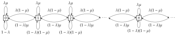
By cutset $\lambda(1-\mu)\pi_{i}=(1-\lambda)\mu\pi_{i+1}$ , $\boldsymbol{\pi}$ exists only on $\lambda<\mu$ when the chain is positively recurrent,

\pi_{i}=\left(1-\frac{\lambda(1-\mu)}{\mu(1-\lambda)}\right)\cdot\left(\frac{% \lambda(1-\mu)}{\mu(1-\lambda)}\right)^{i},

and the chain being null recurrent on $\lambda=\mu$ , being transient on $\lambda>\mu$ .

When we reverse the order, say on new time step with probability $\mu$ the nonempty queue a customer is processed, and a customer will arrive with probability $\lambda$ at the end of the time step, the new Markov chain follows.

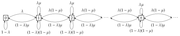
The only difference lies in the empty queue, that follows the vanilla discrete time queue behavior, as the empty queue does not have customers to consume, and either with probability $\lambda$ to accept new customer at the end of the time step, or remain empty with probability $1-\lambda$ .

By cutset, we have

	$\displaystyle\lambda\pi_{0}$	$\displaystyle=(1-\lambda)\mu\pi_{1}$
	$\displaystyle\lambda(1-\mu)\pi_{i}$	$\displaystyle=(1-\lambda)\mu\pi_{i+1},$

hence for $i\geq 1$ ,

\pi_{i}=\frac{\pi_{0}}{1-\mu}\cdot\left(\frac{\lambda(1-\mu)}{\mu(1-\lambda)}% \right)^{i},

and by $\sum_{i\geq 0}\pi_{i}=1$ , we have

\pi_{0}=1-\frac{\lambda}{\mu}.

Therefore, for $i\geq 1$ ,

\pi_{i}=\frac{\pi_{0}}{1-\mu}\cdot\left(\frac{\lambda(1-\mu)}{\mu(1-\lambda)}% \right)^{i},

with the existence condition for $\boldsymbol{\pi}$ being $\lambda<\mu$ , in which case the chain is positively recurrent. ∎

1.7.5 Random Walks on Undirected Graphs

Definition 1.7.73.

A random walk on $G$ is a Markov chain defined by the sequence of moves of a particle between vertices of $G$ . The position of the particle at a particular time step is the state of the chain. If the particle is at vertex $i$ with $d(i)$ outgoing edges, then the probability that the particle follows edge $(i,j)$ to neighboring vertex $j$ is $d(i)^{-1}$ .

Lemma 1.7.74.

A random walk on an undirected graph $G$ is aperiodic iff $G$ is not bipartite, which means there is no 2-coloring such that the endpoints of each edge are colored differently.

Proof.

A graph $G$ being not bipartite means it has cycles of odd length. If a graph $G$ is bipartite and undirected, then the length of the path going back to itself is always even, such that the Markov chain is of period $2$ . Otherwise, undirected $G$ is not bipartite, each vertex has an odd-length path back to itself, then the Markov chain is aperiodic. ∎

Similar to theorem 1.7.53, A random walk on a finite, undirected, connected, and non-bipartite graph $G$ defines a Markov chain that converges to a stationary distribution that is determined by the degree sequences of the graph.

Theorem 1.7.75.

A random walk on a finite, undirected, connected, and non-bipartite $G$ has a stationary distribution $\boldsymbol{\pi}$ where

\pi_{v}=\frac{d(v)}{2\left|E\right|}.

Proof.

Since $\sum_{v\in V}d(v)=2\left|E\right|$ , then $\boldsymbol{\pi}$ defines a proper distribution of particle appearing over $V$ .

On the other hand, by definition of stationary distribution in theorem 1.7.56, for $u\in V$ and its neighbors $\Gamma(u)$ ,

\sum_{v\in\Gamma(u)}\frac{d(v)}{2\left|E\right|}\cdot\frac{1}{d(v)}=\frac{d(u)% }{2\left|E\right|}=\frac{d(u)}{2\left|E\right|}\cdot\sum_{v\in\Gamma(u)}\frac{% 1}{d(u)},

where the second equality holds from $\left|\Gamma(u)\right|=d(u)$ . ∎

Exercise 1.7.76 (Exercise 7.14 [MU17]).

Show that the Markov chain defined by a random walk on a finite, undirected, non-bipartite, connected graph $G$ is time reversible.

Proof.

When $G$ is finite, then theorem 1.7.75 kicks in, by definition of time reversibility in 1.7.63,

\frac{d(v)}{2\left|E\right|}\cdot\frac{1}{d(v)}=\frac{1}{2\left|E\right|}=% \frac{d(u)}{2\left|E\right|}\cdot\frac{1}{d(u)}.

∎

Lemma 1.7.77 (Commute Time).

For $G=(V,E)$ , if $(u,v)\in E$ , the commute time $h_{u,v}+h_{v,u}\leq 2\left|E\right|$ .

Proof.

Let $D$ be the set of directed edges: for every $(u,v)\in E$ , we have 2 directed edges $u\to v$ and $v\to u$ in $D$ .

We can view the random walk over $G$ as a Markov chain of state space $D$ , where the state of the Markov chain at the $t^{\mathrm{th}}$ time step is the direct edge taken by the random walk in its $t^{\mathrm{th}}$ transition. The Markov chain has $2\left|E\right|$ states, and the stationary distribution $\pi_{u\to v}=\left(2\left|E\right|\right)^{-1}$ for all $(u,v)\in E$ , by cutset theorem 1.7.56

\pi_{u\to v}=\frac{1}{d(u)}\sum_{w\in\Gamma(u)}\pi_{w\to u}

for all $(u,v)\in E$ and $\Gamma(u)$ is the set of neighboring vertices of $u$ , $\pi_{u\to v}=\left(2\left|E\right|\right)^{-1}$ is a solution. By theorem 1.7.53,

\pi_{u\to v}=h_{u\to v,u\to v}^{-1}=\left(2\left|E\right|\right)^{-1},

hence $h_{u\to v,u\to v}=2\left|E\right|$ : after taking the directed path $u\to v$ , the expected number of steps to retake $u\to v$ is $2\left|E\right|$ . By Markovian (memoryless) of the random walk, once it reaches $v$ , it forgets about it reaches by $u\to v$ , hence the expected time to start from $v$ and reach $u$ and take $(u,v)$ to $v$ is $2\left|E\right|$ .

Since $h_{u,v}$ will not rule out the walk reaching $v$ without taking $(u,v)$ , then it will not force the walk to go back to $u$ and take $(u,v)$ , even if it reached $v$ before, hence $h_{v,u}+h_{u,v}\leq h_{u\to v,u\to v}=2\left|E\right|$ . ∎

Exercise 1.7.78 (Exercise 7.22 [MU17]).

A cat and a mouse each independently take a random walk on a connected, undirected, non-bipartite graph $G$ . They start at the same time on different nodes, and each makes 1 transition at each time step. The cat eats the mouse if they are ever at the same node at a time step. Let $\left|V\right|=n$ and $\left|E\right|=m$ . Show an upper bound of $O(m^{2}n)$ on the expected time before the cat eats the mouse.

Proof.

Construct a graph $G^{2}$ from $G$ by making vertices $V^{2}=(V,V)$ , and edges $E^{2}$ for all $\left((u_{0},u_{1}),(v_{0},v_{1})\right)$ such that $(u_{0},v_{0})\in E$ and $(u_{1},v_{1})\in E$ . Counting the degrees of each vertices $(a,b)\in V^{2}$ double counts $\left|E^{2}\right|$ , then

2\left|E^{2}\right|^{2}=\sum_{(a,b)\in V^{2}}d(a,b)=\sum_{a\in V}d(a)\sum_{b% \in V}d(b)=4\left|E\right|^{2},

such that $\left|E^{2}\right|=2\left|E\right|^{2}$ .

We show that, for every $(a,b)\in V^{2}$ , there exists paths of $O(\left|V\right|)$ length to a $(v,v)\in V^{2}$ in the connected, undirected, non-bipartite graph. First, for every $u,v\in V$ , the path in between over $G$ is $O(\left|V\right|)$ length. Then, for paths in between $a, v$ and $b, v$ , we use $\ell_{1},\ell_{2}$ to denote the paths lengths,

•

If both $\ell_{1},\ell_{2}$ are even or odd, then there exists path in between $(a,b),(v,v)$ of length $\max(\ell_{1},\ell_{2})=O(\left|V\right|)$ , as the shorter one can keep looping in between $v$ and $u\in\Gamma(v)$ for $2k$ steps, such that they eventually meet at $(v,v)$ .
•

Otherwise, since $G$ is non-bipartite, there exists odd length cycle in $G$ , such that the odd length path can be transformed into an even length path, and the 2 lengths can be calibrated to be the same as previously described. The cycle is of $O(\left|V\right|)$ length, and original paths are $O(\left|V\right|)$ lengths, hence the resulting length is $O(\left|V\right|)$ .

After obtaining such path $\mathbf{s}$ from $(a,b)$ to $(v,v)$ of length $\ell=O(\left|V\right|)$ , we bound $h_{(a,b),(v,v)}$ by

h_{(a,b),(v,v)}\leq h_{(a,b),(v,v)}+h_{(v,v),(a,b)}\leq\sum_{i\in[1,\ell-1]}% \left(h_{(s_{i},s_{i+1})}+h_{(s_{i+1},s_{i})}\right)\leq\ell\cdot 2\left|E^{2}% \right|=4\ell\left|E\right|^{2}.

where the second inequality holds by enforcing the path $\mathbf{s}$ from $(a,b)$ to $(v,v)$ , similar to the idea of lemma 1.7.77, and the third inequality is immediate by lemma 1.7.77. Hence, the expected time $h_{(a,b),(v,v)}=O(\left|E\right|^{2}\left|V\right|)$ . ∎

Definition 1.7.79 (Covering Time).

The covering time of $G=(V,E)$ is the max of all $v\in V$ of the expected time to visit all vertices by a random walk starting from $v$ .

Lemma 1.7.80 (Covering Time Upper Bound).

The covering time $C_{G}$ of $G=(V,E)$ is upper bounded by $2\left|E\right|\left(\left|V\right|-1\right)$ .

Proof.

One can consider traversing all vertices with a MST in $G$ , such that there are $\left|V\right|-1$ directed paths in the MST. Then we bound similarly in lemma 1.7.77 and 1.7.78 by enforcing the paths

C_{G}\leq\sum_{i\in[1,\left|V\right|-1]}\left(h_{v_{i},v_{i+1}}+h_{v_{i+1},v_{% i}}\right)\leq 2\left|E\right|\left(\left|V\right|-1\right).

∎

We introduce Matthew’s theorem, connecting the hitting time $h_{u,v}$ to the covering time. We write $H(n)=\sum_{i\leq n}1/i$ .

Lemma 1.7.81 (Matthews’ Theorem [Mat88]).

The covering time $C_{G}$ of $G=(V,E)$ with $\left|V\right|=n$ is bounded by

H(n-1)\min_{u,v\in V,u\neq v}h_{u,v}\leq C_{G}\leq H(n-1)\max_{u,v\in V,u\neq v% }h_{u,v}.

Proof.

The proof utilizes balls-and-bins model, and the path enforcing technique of lemma 1.7.77 and 1.7.78.

We begin by enforcing a traversal order $\{Z_{i}\}_{i\in[1,n]}$ over $V$ sampled from uniform permutation over $[1,n]$ , write $B$ as the maximal hitting time $h_{u,v}$ for convenience, $T_{i}$ be the first time step when all the first $i$ vertices $Z_{1},\ldots,Z_{i}$ have been visited in the order ⁶⁶6 If $Z_{j}$ are visited for $j\in[1,k]\setminus\{i\}$ , then when $Z_{i}$ is visited, $T_{i}=T_{i+1}=\cdots=T_{k}$ . , and $X_{i}$ be the state of the Markov chain at the $i^{\mathrm{th}}$ time step.

Given all the prior setup, we are interested in the time intervals $\{T_{i}-T_{i-1}\}_{i\in[2,n]}$ . Given the random walk history,

Y_{i}=\operatorname*{\mathbb{E}}\left[T_{i}-T_{i-1}\mid Z_{1},\ldots,Z_{i};X_{% 1},\ldots,X_{T_{i-1}}\right]

for $i\in[2,n]$ ⁷⁷7 Coupon-collector on the first $k$ entries, that does not strictly enforces traverse by the permutation, but enforces by visiting first $k$ entries. , and the expected time to cover the graph starting from $u$ is

C_{G}=\sum_{i\in[2,n]}Y_{i}+\operatorname*{\mathbb{E}}\left[T_{1}\right].

For $T_{1}$ , one has $1/n$ probability having $Z_{1}=u$ , otherwise $u$ is reached by random walk. By conditional expectation,

	$\displaystyle\operatorname*{\mathbb{E}}\left[T_{1}\right]$	$\displaystyle=\operatorname*{\mathbb{E}}\left[T_{1}\mid Z_{1}=u\right]\Pr\left% [Z_{1}=u\right]$
		$\displaystyle+\operatorname*{\mathbb{E}}\left[T_{1}\mid Z_{1}\neq u\right]\Pr% \left[Z_{1}\neq u\right]$
		$\displaystyle\leq\left(1-\frac{1}{n}\right)B,$

where the second inequality holds by $B$ upper bounding the expectation of hitting time, and $T_{1}=0$ when $Z_{1}=u$ .

For $Y_{i}$ , if $i$ has already been visited previously, then $Y_{i}=0$ as $T_{i}=T_{i-1}$ , otherwise $Y_{i}\leq B$ regardless.

Since the permutation $\{Z_{i}\}_{i\in[1,n]}$ is sampled uniformly random and independent of the random walk, then any one of $\{Z_{k}\}_{i\in[1,k]}$ can be the last visited for first $k$ entries with probability $1/k$ ⁸⁸8 $Z_{k}$ being last visited w.r.t. the fixed random walk is only related to $\{Z_{i}\}_{i\in[1,k]}$ , by symmetry of random permutation, the probability is $1/k$ . , and hence

	$\displaystyle\sum_{i\in[2,n]}Y_{i}+\operatorname*{\mathbb{E}}\left[T_{i}\right]$	$\displaystyle\leq\sum_{i\in[2,n]}\frac{1}{i}B+\left(1-\frac{1}{n}\right)B$
		$\displaystyle=\sum_{i\in[1,n-1]}\frac{1}{i}B$
		$\displaystyle=H(n-1)B.$

The lower bound is proven in the same way, by setting $B$ to be the minimal of the expected hitting time. ∎

Exercise 1.7.82 (Exercise 7.24 [MU17]).

A lollipop graph on $n$ vertices is a clique $K_{n/2}$ connected to a $n/2$ long path. $u$ is the node being both clique and path, and $v$ be the other end of the path. Show the $C_{G}$ starting from $v$ is $\Theta(n^{2})$ , and starting from $u$ is $\Theta(n^{3})$ .

Proof.

We bound the covering time from $v$ by enforcing the path from $v$ to $u$ , then to other $x\in K_{n/2}$ . By lemma 1.7.80,

C_{G}\leq h_{v,u}+\sum_{x\in K_{n/2},x\neq u}\left(h_{x,u}+h_{u,x}\right).

For $h_{v,u}$ , let $i\in[1,n/2-1]$ be vertices on the $(u,v)$ path, we have

	$\displaystyle h_{1,u}$	$\displaystyle=\frac{1}{2}\cdot 1+\frac{1}{2}\cdot\left(1+h_{2,u}\right)$
		$\displaystyle\cdots$
	$\displaystyle h_{{n/2-1},u}$	$\displaystyle=\frac{1}{2}\cdot\left(1+h_{{n/2-2},u}\right)+\frac{1}{2}\cdot% \left(1+h_{v,u}\right)$
	$\displaystyle h_{v,u}$	$\displaystyle=1+h_{{n/2-1,u}},$

hence $h_{i,u}=i\cdot(n-i)$ , and $h_{v,u}=n^{2}/4$ .

For $h_{u,x}$ for some $x\in K_{n/2}$ , let $k=n/2$ and $x^{\prime}\neq x$ that $x^{\prime}\in K_{n/2}$ , then

	$\displaystyle h_{u,x}$	$\displaystyle=\frac{1}{k}\cdot 1+\frac{k-2}{k}\cdot\left(1+h_{x^{\prime},x}% \right)+\frac{1}{k}\cdot\left(1+h_{1,x}\right)$
	$\displaystyle h_{x^{\prime},x}$	$\displaystyle=\frac{1}{k-1}\cdot 1+\frac{k-3}{k-1}\cdot\left(1+h_{x^{\prime},x% }\right)+\frac{1}{k-1}\cdot\left(1+h_{u,x}\right)$
	$\displaystyle h_{1,x}$	$\displaystyle=\frac{1}{2}\cdot\left(1+h_{u,x}\right)+\frac{1}{2}\cdot\left(1+h% _{2,x}\right)$
		$\displaystyle\cdots$
	$\displaystyle h_{v,x}$	$\displaystyle=1+h_{n/2-1,x},$

then $h_{u,x}=(2k^{2}+3)/2k=n+3/n$ .

For the rest of hitting time from $x\neq u$ , $x\in K_{n/2}$ , there is a vanilla way of computing by

	$\displaystyle h_{x,u}$	$\displaystyle=\frac{1}{k-1}\cdot 1+\frac{k-2}{k-1}\cdot\left(1+h_{x^{\prime},u% }\right)$
	$\displaystyle h_{x^{\prime},u}$	$\displaystyle=\frac{1}{k-1}\cdot 1+\frac{k-2}{k-1}\cdot\left(1+h_{x^{\prime},u% }\right),$

then $h_{x,u}=h_{x^{\prime},u}=k-1$ .

Another way of deriving $h_{x,u}$ is by taking advantage of theorem 1.7.75, that the lollipop graph is non-bipartite as $K_{n/2}$ has odd length cycle, then

\pi_{u,u}^{-1}=\frac{2\left|E\right|}{d(u)}=h_{u,u}=\frac{1}{d(u)}\sum_{w\in% \Gamma(u)}\left(h_{w,u}+1\right)=1+\frac{1}{k}\sum_{w\in\Gamma(u)}h_{w,u},

where $d(u)=\left|\Gamma(u)\right|=k$ , hence $\sum_{w\in\Gamma(u)}h_{w,u}=2\left|E\right|-k$ . Since $\left|E\right|=k(k+1)/2$ , and $h_{1,u}=n-1=2k-1$ , hence

\sum_{w\in\Gamma(u),w\neq 1}h_{w,u}=2\left|E\right|-k-h_{1,u}=(k-1)^{2}.

Therefore, the covering time from $v$ is $\Theta(n^{2})$ .

To derive the $C_{G}$ from $u$ , $h_{u,v}$ is upper bounding the covering time for the path part, then

C_{G}\leq h_{u,v}+\sum_{x\in K_{n/2},x\neq u}\left(h_{x,u}+h_{u,x}\right),

and we have the formulas

	$\displaystyle h_{x,v}$	$\displaystyle=\frac{1}{k-1}\cdot\left(1+h_{u,x}\right)+\frac{k-2}{k-1}\cdot% \left(1+h_{x,v}\right)$
	$\displaystyle h_{u,v}$	$\displaystyle=\frac{1}{k}\cdot\left(1+h_{1,v}\right)+\frac{k-1}{k}\cdot\left(1% +h_{x,v}\right)$
	$\displaystyle h_{1,v}$	$\displaystyle=\frac{1}{2}\cdot\left(1+h_{u,v}\right)+\frac{1}{2}\cdot\left(1+h% _{2,v}\right)$
		$\displaystyle\cdots$
	$\displaystyle h_{n/2-1,v}$	$\displaystyle=\frac{1}{2}\cdot 1+\frac{1}{2}\cdot\left(1+h_{n/2-2,v}\right),$

then $h_{k-i,v}=i\cdot(k^{2}+k-i)$ , and hence $h_{u,v}=k^{3}$ , which explains $C_{G}$ from $u$ is $\Theta(n^{3})$ . ∎

Exercise 1.7.83 (Exercise 7.26 [MU17]).

Let $n$ equidistant points be marked on a circle. WLOG, think of the points as being labeled clockwise from $0$ to $n-1$ . Initially, a wolf begins at 0 and there is one sheep at each of the remaining $n-1$ points. The wolf takes a random walk on the circle. For each step, it moves with probability $1/2$ to one neighboring point and with probability $1/2$ to the other neighboring point. At the first visit to a point, the wolf eats a sheep if there is still one there. Which sheep is most likely to be the last eaten?

Proof.

Brain teaser. Say for any sheep $j\in[1,n-1]$ is eaten last, then view this as a Gambler’s Ruin example 1.7.51 by states $j,j+1\cdots n-1,0,1,\cdots,j-1,j$ and absorb at both $j$ ’s. Now the requirement is, visit all states before absorbing.

Visiting $j+1$ first is mutually exclusive with visiting $j-1$ first, and hence the rest is visiting $j+1$ or $j-1$ , then absorb to the $j$ on the other end, which is of probability $1/(n-1)$ in total.

Such $1/(n-1)$ probability holds for any $j\in[1,n-1]$ , and hence all sheeps eaten last is equal probability. ∎

Exercise 1.7.84 (Exercise 7.30 [MU17]).

Let $(u,v)$ be an edge in a hypercube of $N=2^{n}$ nodes.

•

Prove the expected time between the traversal of $(u,v)$ edge is $n N$ .
•

We consider the time between transitions from $u$ to $v$ in a different way. After moving from $u$ to $v$ , the walk must first return to $u$ . When it returns to $u$ , the walk might next move to $v$ , or it might move to another neighbor of $u$ , in which case it must return to $u$ again before moving to $v$ for there to be a transition from $u$ to $v$ .

Use symmetry and the above description to prove the following recurrence:

$Nn=\sum_{i\geq 1}\frac{1}{n}\left(\frac{n-1}{n}\right)^{i-1}(i(h_{u,v}+1))=n(h% _{u,v}+1).$
•

Conclude that $h_{u,v}=N-1$ .
•

Using the result on the hitting time of adjacent vertices and Matthews’ theorem, show the cover time is $O(Nn^{2})$ .
•

As a much more challenging problem, try to prove that the maximum hitting time between any two vertices for the random walk on the hypercube is $O(N)$ , and that the cover time is correspondingly $O(Nn)$ .

Proof.

Each vertex in an $n$ -dimensional hypercube has $n$ edges, then $2\left|E\right|=nN$ . By lemma 1.7.77,

h_{u\to v,u\to v}=2\left|E\right|=nN.

To derive $h_{u\to v,u\to v}$ again from geometric distribution, consider $u$ going to $v$ , or $n-1$ other neighbors in $\Gamma(u)\setminus\{v\}$ . It takes one step to go from $u$ to any $w\in\Gamma(u)$ . To get back to $u$ from $w\in\Gamma(u)$ , $h_{w,u}=h_{v,u}=h_{u,v}$ by symmetry.

Hence, a trial contains going back from neighbor $w\in\Gamma(u)$ , then depart from $u$ to one of the neighbors in $\Gamma(u)$ . By Markovian of random walk, the probability of going from $u$ to $v$ is $n^{-1}$ , hence the expected steps to take $(u,v)$ is

\sum_{i\geq 1}\frac{1}{n}\left(\frac{n-1}{n}\right)^{i-1}\cdot i(h_{u,v}+1)=n(% h_{u,v}+1).

By prior result on $h_{u\to v,u\to v}$ by lemma 1.7.77, we conclude that $h_{u,v}=N-1$ .

Consider any $p,q\in V$ for the hypercube, that $(p,q)\notin E$ . Similar to 1.7.78, we upper bound by

h_{p,q}\leq\sum_{(a,b)\in P}h_{a,b}=O(Nn),

where there is a path of length $O(n)$ connecting $p$ and $q$ , as there are at most $O(n)$ bits different in between $p$ and $q$ . By lemma 1.7.81, $H(N-1)=O(n)$ , hence the covering time is upper bounded by $O(n^{2}N)$ .

For departing from $u$ , we can model the hitting time to $v$ by the Hamming distance as follows.

Then the linear system for the hitting time is

	$\displaystyle h_{0,n}$	$\displaystyle=1+h_{1,n}$
	$\displaystyle h_{i,n}$	$\displaystyle=1+\frac{i}{n}\cdot h_{i-1,n}+\frac{n-i}{n}\cdot h_{i+1,n}$
	$\displaystyle h_{n-1,n}$	$\displaystyle=1+\frac{n-1}{n}\cdot h_{n-2,n},$

and let $d_{i}=h_{i,n}-h_{i+1,n}$ with $d_{n-1}=h_{n-1,n}$ , then

	$\displaystyle d_{0}$	$\displaystyle=1$
	$\displaystyle(n-i)d_{i}$	$\displaystyle=n+id_{i-1}.$

Since

	$\displaystyle(n-i)\binom{n-1}{i-1}$	$\displaystyle=i\binom{n-1}{i}$
	$\displaystyle n\binom{n-1}{i}$	$\displaystyle=(n-i)\binom{n}{i},$

then

	$\displaystyle(n-i)\binom{n-1}{i}d_{i}$	$\displaystyle=n\binom{n-1}{i}+i\binom{n-1}{i}d_{i-1}$
		$\displaystyle=(n-i)\binom{n}{i}+(n-i)\binom{n-1}{i-1}d_{i-1},$

and eventually

s_{i}=\binom{n-1}{i}d_{i}=\binom{n}{i}+\binom{n-1}{i-1}d_{i-1}=\binom{n}{i}+s_% {i-1}.

Since $s_{0}=1$ , hence

s_{k}=\sum_{i\in[0,k]}\binom{n}{i}=2^{n}-\sum_{i\in[k+1,n]}\binom{n}{k},

and

d_{k}=\binom{n-1}{k}^{-1}\sum_{i\in[0,k]}\binom{n}{i}=\binom{n-1}{k}^{-1}\left% (2^{n}-\sum_{i\in[k+1,n]}\binom{n}{k}\right),

and finally

	$\displaystyle h_{0,n}$	$\displaystyle=\sum_{k\in[0,n-1]}d_{k}$
		$\displaystyle=\sum_{k\in[0,n-1]}\binom{n-1}{k}^{-1}\sum_{i\in[0,k]}\binom{n}{i}.$

Since $d_{n-1}=2^{n}-1$ , $d_{n-2}\leq 2^{n}/(n-1)$ , and

	$\displaystyle\sum_{k\in[2,n-3]}\binom{n-1}{k}^{-1}$	$\displaystyle\leq\sum_{k\in[2,n-3]}\binom{n-1}{2}^{-1}$
		$\displaystyle=\frac{2(n-4)}{(n-1)(n-2)}=O(n^{-1}).$

then $h_{0,n}=O(N)$ . By lemma 1.7.81 again, the covering time is $O(nN)$ . ∎

1.7.6 Parrondo’s Paradox

Parrondo’s paradox shows that, sometimes 2 losing games combined together makes a winning game.

•

Consider a game $A$ with a biased coin $A$ , winning with probability $p_{A}$ and losing with probability $1-p_{A}$ .
•

Consider a game $B$ , that the coin flipped depends on the state of the game.
Let $w$ be the number of games won so far, and $\ell$ be the number of games lost so far, then $w-\ell$ is the winning.
- –
  
  If $w-\ell\equiv 0\mod 3$ , then use coin $B$ winning with probability $p_{B}$ and losing with probability $1-p_{B}$ .
- –
  
  Otherwise, use coin $C$ winning with probability $p_{C}$ and losing with probability $1-p_{C}$ .

To show whether game $B$ is winning or losing, we use the following lemma.

Lemma 1.7.85.

For any sequence $s$ of moves that starts at $0$ and ends at $3$ before reaching $-3$ , let $f(s)$ be a 1-to-1 mapping to $s$ such that $f(s)$ negates every number starting from the last 0 in the sequence $s$ , then

\frac{\Pr\left[s\text{ occurs}\right]}{\Pr\left[f(s)\text{ occurs}\right]}=% \frac{p_{B}p_{C}^{2}}{(1-p_{B})(1-p_{C})^{2}}.

Proof.

We can view the game $B$ by a Markov chain over $[-3,3]$ that starts from $0$ , with $\pm 3$ being 2 absorbing states. Similar to the Gambler’s ruin argument in example 1.7.51, if it is more likely to reach $-3$ before reaching $3$ , then the game is a losing game.

Now consider the 1-to-1 mapping. Let

•

$a_{1}$ be the number of moves $0\to 1$ ,
•

$a_{2}$ be the number of moves from $0\to-1$ ,
•

$a_{3}$ be the number of moves $1\to 2$ , $2\to 3$ , $-2\to-1$ , $-1\to 0$ ,
•

$a_{4}$ be the number of moves $2\to 1$ , $1\to 0$ , $-1\to-2$ , $-2\to-3$

in $s$ . Then

\Pr\left[s\text{ occurs}\right]=p_{B}^{a_{1}}(1-p_{B})^{a_{2}}p_{C}^{a_{3}}(1-% p_{C})^{a_{4}}.

Consider $f(s)$ reaching $-3$ before reaching $3$ that is 1-to-1 mapped to $s$ .

•

Since the first move after last 0 in $s$ is $0\to 1$ , then the first move after last 0 in $f(s)$ is $0\to-1$ , hence $a_{1}^{\prime}=a_{1}-1$ . By symmetry of $a_{1}+a_{2}=a_{1}^{\prime}+a_{2}^{\prime}$ , we have $a_{2}^{\prime}=a_{2}+1$ .
•

After the last $0\to 1$ in $s$ , there is no $1\to 0$ moves. The remaining moves in $s$ are $1\to 2$ , $2\to 1$ , and $2\to 3$ . For $f(s)$ , the remaining moves are $-1\to-2$ , $-2\to-1$ , and $-2\to-3$ .

All the moves $-1\to-2$ then $-2\to-1$ in $f(s)$ are self-cancelling, symmetric to the $1\to 2$ then $2\to 1$ on $s$ side.

What remains is $1\to 2\to 3$ in $s$ , and $-1\to-2\to-3$ in $f(s)$ . Hence, $a_{3}^{\prime}=a_{3}-2$ , and $a_{4}^{\prime}=a_{4}+2$ .

Therefore,

\Pr\left[f(s)\text{ occurs}\right]=p_{B}^{a_{1}-1}(1-p_{B})^{a_{2}+1}p_{C}^{a_% {3}-2}(1-p_{C})^{a_{4}+2},

and the ratio $\eta=p_{B}p_{C}^{2}(1-p_{B})^{-1}(1-p_{C})^{-2}$ . ∎

Suppose $p_{A}=0.49$ , $p_{B}=0.09$ , $p_{C}=0.74$ , then both game $A$ and game $B$ are both losing, as $\eta\approx 0.8$ .

However, with a fair coin $D$ with $p_{D}=0.5$ , we combine the game by winning on coin $D$ plays game $A$ , and losing on coin $D$ plays game $B$ . In this case, $p_{B}^{\prime}=(p_{A}+p_{B})/2$ and $p_{C}^{\prime}=(p_{A}+p_{C})/2$ , and eventually $\eta>1$ .

The difference lies in the fair coin $D$ breaks the structure of game $B$ , that is rather likely to lose on any game with $w-\ell\equiv 0\mod 3$ . If one managed to get over the barrier in game $B$ with game $A$ , which is close to a fair game, then it is likely to win the next 2 games.

1.7 Markov Chains and Random Walks

1.7.1 Stirling’s Formula

Lemma 1.7.1 (Stirling’s Formula).

Proof.

Lemma 1.7.2 (log⁡(x+1) bounds [Top07]).

Corollary 1.7.3.

Proof.

1.7.2 Markov Chains and Classification of States

Definition 1.7.4.

Exercise 1.7.5 (Exercise 7.2 [MU17]).

Proof.

Lemma 1.7.6 (2-SAT randomized algorithm expected runtime [Pap91]).

Proof.

Theorem 1.7.7.

Proof.

Exercise 1.7.8 (Exercise 7.6 [MU17]).

Proof.

Exercise 1.7.9 (Exercise 7.7 [MU17]).

Proof.

Exercise 1.7.10 (Exercise 7.8 [MU17]).

Proof.

Exercise 1.7.11 (Exercise 7.9 [MU17]).

Proof.

Exercise 1.7.12 (Exercise 7.10 [MU17]).

Proof.

Theorem 1.7.13 (Chapman-Kolmogorov Equation).

Proof.

Definition 1.7.14.

Definition 1.7.15.

Lemma 1.7.16.

Definition 1.7.17.

Definition 1.7.18.

Exercise 1.7.19 (Exercise 7.15 [MU17]).

Proof.

Corollary 1.7.20.

Proof.

Definition 1.7.21.

Corollary 1.7.22.

Proof.

Corollary 1.7.23.

Proof.

Remark 1.7.24.

Example 1.7.25.

Theorem 1.7.26.

Proof.

Lemma 1.7.27.

Proof.

1.7.3 Strong Law of Large Numbers (SLLN)

Theorem 1.7.28 (Kolmogorov SLLN).

Definition 1.7.29.

Lemma 1.7.30 (Borel-Cantelli Lemma [Fel68a]).

Proof.

Remark 1.7.31.

Proof.

Lemma 1.7.32.

Lemma 1.7.33.

Lemma 1.7.34.

Proof.

Proof.

Lemma 1.7.35 (Etemadi Inequality [Ete81]).

Proof.

Corollary 1.7.36.

Proof.

Definition 1.7.37 (Stopping Time).

Definition 1.7.38 (Strong Markov Property for Discrete-Time Markov Chains).

Theorem 1.7.39.

Proof.

Theorem 1.7.40 (SLLN for Markov chains).

Proof.

Theorem 1.7.41 (Bounded Convergence Theorem).

Corollary 1.7.42 (Cesàro Limit of Return Probability).

Proof.

Lemma 1.7.43.

Proof.

1.7.4 Stationary Distributions

Definition 1.7.44.

Example 1.7.45.

Definition 1.7.46.

Corollary 1.7.47.

Lemma 1.7.48 (Ergodic Limit of Return Probability).

Lemma 1.7.2 ( $\log(x+1)$ bounds [Top07]).